How to avoid this kind of numerical error caused by extreme parameters when using NDSolve?

Question

Here I use a one-dimensional heat conduction equation as the example. I found that when the thermal diffusion coefficient is small enough, Mathematica will give a result against the second law of thermodynamics:

fun[k_] := (a = NDSolve[{D[tes[t, x], t] == k D[tes[t, x], x, x], 
　　　　　　　　　　    　　tes[t, 0] == t, tes[t, 1] == 0, tes[0, x] == 0}, 
　　　　　　　　　　   　　{tes[t, x]}, {t, 0, 1}, {x, 0, 1}]; 
　　　　　　Plot[(tes[t, x] /. a) /. t -> 1, {x, 0, 1}, PlotRange -> All]);
fun[1]
fun[10^-3]
fun[10^-6]

Here's the result:

Graph 1

Graph 2

Graph 3

The circled part in Graph 3 is the crux: this wave is unreasonable in the view of physics. So, how to avoid this if I have to use this kind of parameters?

Answer 1

It looks you need to use other NDSolve options to control the spatial grid size to help NDSolve a little.

Trying things, found that by increasing the grid size, now this effect you showed goes away.

Grid size needs to be much smaller when the diffusion coefficient is very small since you are effectively in $\lim{k \to 0}$ now solving $\frac{\partial u}{\partial t} = k \left( \frac{\partial^2 u}{\partial x^2} \right)$ as $ \frac{\partial u(x,t)}{\partial t}=0$.

Using NDSolve with "MethodOfLines" options and increasing the "MaxPoints" helped get rid of this problem. There might be other and better options to try.

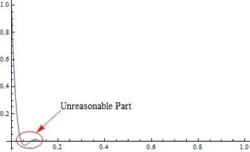
This function below takes the number of spatial grid points you want to use. The smaller $k$ is, the larger the number of grid points need to be (i.e smaller grid size) to get rid of that kink near the left boundary you had.

 Manipulate[
 fun[k, lim, grid],
 {{k, 1, "k"}, 0.000001, 1, 0.000001, Appearance -> "Labeled"},
 {{grid, 39, "grid points"}, 39, 999, 2, Appearance -> "Labeled"},
 {{lim, 1, "plot x limit"}, 0.01, 1, 0.01, Appearance -> "Labeled"},

 SynchronousUpdating -> False,
 ContinuousAction -> False,
 SynchronousInitialization -> True,
 Initialization :>
  {
   fun[k_, lim_, nPoints_] := Module[{u, t, x, sol, ic, bc},
     bc = {u[t, 0] == t, u[t, 1] == 0};
     ic = u[0, x] == 0;

     sol = 
      First@NDSolve[
        Flatten[{D[u[t, x], t] == k D[u[t, x], x, x], ic, bc}],
        {u[t, x]}, {t, 0, 1}, {x, 0, lim},
        Method -> {"MethodOfLines",              
          "SpatialDiscretization" -> {"TensorProductGrid", 
            "MaxPoints" -> nPoints, "MinPoints" -> nPoints},
          Method -> "Adams"}, MaxSteps -> Infinity];

     Plot[(u[t, x] /. sol) /. t -> 1, {x, 0, lim},
      PlotRange -> All, ImageSize -> 300, Frame -> True, 
      ImageMargins -> {{30, 10}, {20, 20}}]
     ]
   }
 ]

which gives

Answer 2

This is not meant to be an alternative answer but rather a reminder about another potential source of such overshootings: as mentioned in my comment I believe that the interpolating function with order 3 that is created from the numerical solution calculated at the gridpoints is a potential source of such overshootings. It looks to me that much of the "wrong" behaviour that can be seen in the plot doesn't come from an error or inaccuracy from NDSolve but is just an artifact of the interpolation. As I have no insight in the code that does the interpolation and no time for a deep investigation that's just a guess. But I would strongly recomment to keep this in mind as a potential source of such errors when trying to understand results you get from NDSolve. I usually start with extracting the values at the gridpoints in such cases, e.g. as shown here:

With[{k = 10^-6},
  res = tes /. NDSolve[{
       D[tes[t, x], t] == k D[tes[t, x], x, x],
       tes[t, 0] == t,
       tes[t, 1] == 0,
       tes[0, x] == 0
       },
      {tes}, {t, 0, 1}, {x, 0, 1}
      ][[1]]
  ];

Show[
 Plot[res[1, x], {x, 0, 1}, Frame -> True, PlotRange -> All], 
 ListPlot[{#, res[1, #]} & /@ (res@"Coordinates")[[2]], 
  PlotRange -> All, Frame -> True, Mesh -> True, PlotStyle -> Red]
 ]

It might also be instructive to look at explicit values on the gridpoints, e.g.:

Min[res[1, #] & /@ (res@"Coordinates")[[2]]]

(*
==> -0.0000239294
*)

I've seen a comment of ruebenko and think he might be able to share some insight about whether my guess is reasonable or completely off, so I hope he is following this and will make a comment...