Plot electric potential and field

Question

I am trying to plot the electric potential of a dielectric cylinder along with its field. The potential is a piecewise function:

F[r_, f_] := 
 Piecewise[{{-2 e r Cos[f]/(1 + er), 
0 <= r < a}, {-e r Cos[f] + (er - 1)*a^2 *e*r^(-1)*Cos[f], 
r >= a}}](*electorstatic pottential*)
e = 500;(*outer electric field*)
a = 0.02;(*cylinder's radius*)
er = 2;(*relevant acceptance*)

What's the best way to plot this function (potential), with its derivative (electric field)?

I tried to plot it using ContourPlot, but it doesn't look nice (I am not a Mathematica expert apparently)

ContourPlot[-2 e r Cos[f]/(1 + er), {r, 0, a}, {f, 0, 2 Pi}]
ContourPlot[-e r Cos[f] + (er - 1)*a^2 *e*r^(-1)*Cos[f], {r, a, 
2 a}, {f, 0, 2 Pi}]
Show[%, %%]

What I am trying to achieve is a sophisticated plot, with the cylinder at the origin, where the equipotential lines and the electric field lines will be plotted. I found something like that on the net (specifically the page "Gradient field plots in Mathematica"), but I don't know how to modify it...

gradientFieldPlot[f_, rx_, ry_, opts : OptionsPattern[]] := 
 Module[{img, cont, densityOptions, contourOptions, frameOptions, 
   gradField, field, plotRangeRule, rangeCoords}, 
  densityOptions = 
   Join[FilterRules[{opts}, 
     FilterRules[Options[DensityPlot], 
      Except[{Prolog, Epilog, FrameTicks, PlotLabel, ImagePadding, 
        GridLines, Mesh, AspectRatio, PlotRangePadding, Frame, 
        Axes}]]], {PlotRangePadding -> None, Frame -> None, 
     Axes -> None, AspectRatio -> Automatic}];
  contourOptions = 
   Join[FilterRules[{opts}, 
     FilterRules[Options[ContourPlot], 
      Except[{Prolog, Epilog, FrameTicks, PlotLabel, Background, 
        ContourShading, PlotRangePadding, Frame, Axes, 
        ExclusionsStyle}]]], {PlotRangePadding -> None, Frame -> None,
      Axes -> None, ContourShading -> False}];
  gradField = ComplexExpand[{D[f, rx[[1]]], D[f, ry[[1]]]}];
  field = 
   DensityPlot[Norm[gradField], rx, ry, 
    Evaluate@Apply[Sequence, densityOptions]];
  img = Rasterize[field, "Image"];
  plotRangeRule = FilterRules[Quiet@AbsoluteOptions[field], PlotRange];
  cont = If[
    MemberQ[{0, 
      None}, (Contours /. FilterRules[{opts}, Contours])], {}, 
    ContourPlot[f, rx, ry, Evaluate@Apply[Sequence, contourOptions]]];
  frameOptions = 
   Join[FilterRules[{opts}, 
     FilterRules[Options[Graphics], 
      Except[{PlotRangeClipping, PlotRange}]]], {plotRangeRule, 
     Frame -> True, PlotRangeClipping -> True}];
  rangeCoords = Transpose[PlotRange /. plotRangeRule];
  Apply[Show[
     Graphics[{Inset[
        Show[SetAlphaChannel[img, 
          "ShadingOpacity" /. {opts} /. {"ShadingOpacity" -> 1}], 
         AspectRatio -> Full], rangeCoords[[1]], {0, 0}, 
        rangeCoords[[2]] - rangeCoords[[1]]]}], cont, 
     StreamPlot[gradField, rx, ry, 
      Evaluate@FilterRules[{opts}, StreamStyle], 
      Evaluate@FilterRules[{opts}, StreamColorFunction], 
      Evaluate@FilterRules[{opts}, StreamColorFunctionScaling], 
      Evaluate@FilterRules[{opts}, StreamPoints], 
      Evaluate@FilterRules[{opts}, StreamScale]], ##] &, 
   frameOptions]]

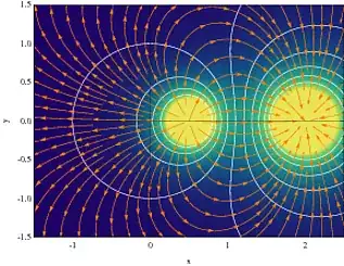
This can be run like that

gradientFieldPlot[(y^2 + (x - 2)^2)^(-1/
    2) - (y^2 + (x - 1/2)^2)^(-1/2)/2, {x, -1.5, 2.5}, {y, -1.5, 
  1.5}, PlotPoints -> 50, ColorFunction -> "BlueGreenYellow", 
 Contours -> 10, ContourStyle -> White, Frame -> True, 
 FrameLabel -> {"x", "y"}, ClippingStyle -> Automatic, Axes -> True, 
 StreamStyle -> Orange]

And the amazing output is

What I would like to do is

Yes, you got that from my web site. I'll be back in a few minutes... — Jens, Jan 05 '13 at 19:05
you could start from ContourPlot[-2 e r Cos[f]/(1 + er), {r, 0, a}, {f, 0, 2 Pi}, ContourShading -> False, ContourStyle -> Red]; ContourPlot[-e r Cos[f] + (er - 1)a^2er^(-1)Cos[f], {r, 0, a}, {f, 0, 2 Pi}, ContourShading -> False, ContourStyle -> Blue]; Show[{%, %%}] and get (http://i.stack.imgur.com/Lp1Zo.png) — chris, Jan 05 '13 at 19:06
@chris: Actually I am trying to do something like this(please check my edited question). — Thanos, Jan 05 '13 at 19:21
If you quote third-party code in your posts (especially when it does not originate on a StackExchange site), please remember to provide a full citation. In addition to being required under the StackExchange terms and conditions, this is because you grant readers a copyright licence to anything you post. If you lack the right to offer such a licence but don't clearly indicate this fact, it could lead to a copyright dispute. — Oleksandr R., Jan 05 '13 at 21:03
@OleksandrR. Thanks for the reminder - I think that gives me the excuse to I edit the question to put my link in now... — Jens, Jan 05 '13 at 21:41

Jens · Accepted Answer · 2013-01-05T19:46:45.557

25

I'll just address the technical plotting aspect of the question.

The problem is that your cylinder potential is intended to be a function of polar coordinates r and f, but to plot it in Cartesian space you have to convert to x and y first. This is done as follows:

pot[r_, f_] := 
 Piecewise[{{-2 e r Cos[f]/(1 + er), 
    0 <= r < a}, {-e r Cos[f] + (er - 1)*a^2*e*r^(-1)*Cos[f], 
    r >= a}}](*electorstatic pottential*)
e = 500;(*outer electric \
field*)a = 0.02;(*cylinder's radius*)er = 2;

gradientFieldPlot[
 pot[Sqrt[x^2 + y^2], ArcTan[x, y]], {x, -.2, .2}, {y, -.2, .2}, 
 PlotPoints -> 50, ColorFunction -> "BlueGreenYellow", Contours -> 10,
  ContourStyle -> White, Frame -> True, FrameLabel -> {"x", "y"}, 
 ClippingStyle -> Automatic, Axes -> True, StreamStyle -> Orange]

plot

The colors represent the field strength, and the orange lines are the field lines.

I called the potential pot instead of F.

Since your cylinder is so small, we should zoom in even more:

gradientFieldPlot[
 pot[Sqrt[x^2 + y^2], ArcTan[x, y]], {x, -.05, .05}, {y, -.05, .05}, 
 PlotPoints -> 50, ColorFunction -> "BlueGreenYellow", Contours -> 10,
  ContourStyle -> White, Frame -> True, FrameLabel -> {"x", "y"}, 
 ClippingStyle -> Automatic, Axes -> True, StreamStyle -> Orange]

plot2

So everything looks as expected for a dielectric cylinder in the homogeneous external field of a capacitor. The equipotential lines (white) are completely flat inside the cylinder, corresponding to a uniform field. The highest field strength is at the "poles" of the dielectric cylinder facing the (far-away) capacitor plates.

edited Jan 05 '13 at 19:46

answered Jan 05 '13 at 19:28

Jens

97,245
7
213
499

@Jens: You are awsome proffessor! That was exactly what I was trying to do! Thank you very much for this very pretty plot! WOW!!! – Thanos Jan 05 '13 at 20:12
@Jens: I was trying to add a legend using PlotLegend -> {"pottential", "field"} inside gradientfieldplot's argument, but nothing showed up(I have already included Needs["PlotLegends"]`). – Thanos Jan 05 '13 at 20:36
1

If you don't have version 9 yet, then Mathematica's PlotLegends package should be avoided like the plague. Instead, in this case perhaps the easiest is to add the PlotLabel option to gradientFieldPlot. E.g., like this: PlotLabel->Framed[Style["Potential (white) and field (orange and background)",Larger,GrayLevel[.3],FontFamily->"Helvetica"],FrameStyle->None,Background->Lighter[Orange],RoundingRadius->6]] – Jens Jan 05 '13 at 22:13
@Jens: I ended there, before I see your comment :(... You are right about Legend-it has issues on v8.0.0. Is there a way to plot a legend illustrating the color scale? Or perhaphs is there a way to plot the whole solution in 3D? – Thanos Jan 06 '13 at 07:51
Hello, I hope you are still active. I was attempting to do this same process for my electrostatics homework, and I was running into issues with mathematica syntax. It doesn't appear that I can copy and paste this code to run, even if I re-enter line by line. I am curious if you think this is because of an outdated version or if I am experiencing a syntax issue I just cant find. – Mike H Oct 19 '21 at 03:16
@MikeH My guess is that you've some global variables that interfere with the plot. Try starting a new session or wrapping the plot command in Module[{x,y}, ...] to protect the dummy variables x and y. – Jens Oct 20 '21 at 16:33
1

That was indeed the problem, and I eventually figured it out. I very much appreciate you coming back and taking the time to help, and thank you very much for your amazing implementation. I made some really neat plots, and to be honest it was my favorite thing to procrastinate my work with for the better part of the time since then. Thank you! – Mike H Nov 01 '21 at 14:20

Plot electric potential and field

1 Answers1

Linked