Voronoi diagrams for generators other than points

Question

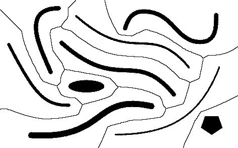
Any suggestions on how to determine a Voronoi diagram for sites other than points, as e.g. in the picture below?

The input is a raster image.

Answer 1

Obtain the image:

i = Import["https://i.stack.imgur.com/iab6u.png"];

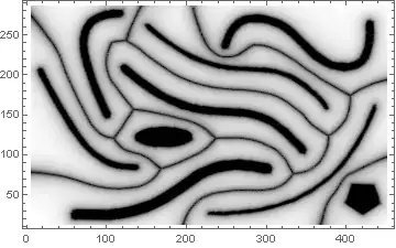
Compute the distance transform:

k = DistanceTransform[ColorNegate[i]] // ImageAdjust;
ReliefPlot[Reverse@ImageData[k]] (* To illustrate *)

Identify the "peaks," which must bound the Voronoi cells:

l = ColorNegate[Binarize[ColorNegate[LaplacianGaussianFilter[k, 2] // ImageAdjust]]];

Clean the result and identify its connected components (the cells):

m = Erosion[Dilation[MorphologicalComponents[l] // Colorize, 2], 1];

Show this with the original features:

ImageMultiply[m, ColorNegate[i]]

Edit

A cleaner solution--albeit one that takes substantially more processing time--exploits WatershedComponents (new in Version 8):

l = WatershedComponents[k];
m = Dilation[MorphologicalComponents[l] // Colorize, 1] (* Needs little or no cleaning *)
ImageMultiply[m, ColorNegate[i]] (* As before *)

I like this one better, but fear it might take too much processing for large complex images.

Answer 2

Here is a Nearest-based method. This is quite similar to what @Mr. Wizard did for approximating 3D (ordinary) Voronoi.

comps     = MorphologicalComponents[img];
cmap      = Flatten[MapIndexed[#2 -> #1 &, comps, {2}]];
comparray = DeleteCases[cmap, _ -> 0];
nf        = Nearest[comparray];

Now we build the table giving Voronoi components.

Timing[
 voronoi2 =
  Array[
   First @ nf[{##}] &,
   Length /@ {comps, comps[[1]]}
  ];
]

(* Out[138]= {0.640000, Null} *)

The picture:

MatrixPlot[voronoi2 + comps, ColorFunction -> "BrightBands", ImageSize -> 500]

Answer 3

OK, you can get the Voronoi diagram using raster-graphics tricks, but what if you want to do it the old-fashioned way?

Download the graphic from the net and parse its components:

img = Import["https://i.stack.imgur.com/iab6u.png"];
morph = MorphologicalComponents[img];
boundary = 
  N[{{0, 0}, {#1, 0}, {#1, #2}, {0, #2}} & @@ (ImageDimensions[img] + 
      1)];
comps = (boundary[[-1]] + {1, -1} Reverse[#] & /@ 
     Position[morph, #]) & /@ Range[Max[morph]];

Take the hulls of the solid shapes. You don't have to do this, but it should make things faster.

hulls = Parallelize[
  Function[set, 
    Cases[set, 
     x_ /; Count[
        MemberQ[set, x + #] & /@ 
         DeleteCases[Tuples[{-1, 0, 1}, {2}], {0, 0}], True] <= 5]] /@
    comps];

Deploy ComputationalGeometry! Start with the Delaunay triangulation, and then get the bounded diagram. (I had to cheat here. Due to some badly conditioned matrices, BoundedDiagram blows up if the boundary is too close.)

Needs["ComputationalGeometry`"]
del = DelaunayTriangulation[pts = N[Join @@ hulls]];
vor = BoundedDiagram[
  boundary /. {0. -> -400., x_?Positive :> x + 400}, pts, del];

Now we just need to paste these back together. This function will fuse adjacent polygons.

fuse[p_, q_] := 
 Module[{l = Intersection[p, q], al, nal, qrot, prot, qdrop}, 
  al = Alternatives @@ l; 
  nal = Except[Alternatives @@ l]; {qrot, prot} = 
   RotateLeft[#, (-Length[l] + 
          Position[
           Differences@Position[#, Alternatives @@ l] - 
            1, {_Integer?
             Positive}] /. {} -> {{Min[
              Position[#, Alternatives @@ l]] - 1}})[[1, 
       1]]] & /@ {DeleteDuplicates[q], p};
  If[Length[DeleteDuplicates[q]] == Length[l], 
   qrot = Take[prot, Length[l]]];
  qdrop = Drop[RotateLeft[qrot], Length[l] - 2];
  prot /. {al .., A : nal ...} :> 
    Join[If[Take[prot, Length[l]] =!= Take[qrot, Length[l]], Identity,
        Reverse][qdrop], {A}]]

mergevor = {vor[[1]], 
  MapIndexed[
   Function[{span, i}, {i[[1]], 
     Fold[fuse, First[#], Rest[#]] &@
      SortBy[vor[[2, Span @@ (span + {1, 0})]], 
        N@Norm[pts[[#[[1]]]] - pts[[vor[[2, span[[1]] + 1, 1]]]]] &][[
       All, 2]]}], 
   Partition[Prepend[Accumulate[Length /@ hulls], 0], 2, 1]]}

And we're done:

Graphics[MapThread[{Hue[#1/Length[hulls]], Opacity[0.5], 
    Polygon[mergevor[[1, #3]]], Opacity[1], PointSize[0.01], 
    Point[#2]} &, {Range[Length[hulls]], hulls, 
   mergevor[[2, All, 2]]}], 
 PlotRange -> ({0, #} & /@ ImageDimensions[img])]

Answer 4

While I cannot match @whuber's simple elegance, I will show a bit of brutishness by using Fast Marching from scratch. This finds distances from a specified boundary. I'll modify it so that, for each pixel, it returns the value of the nearest boundary components.

The code is a bit long but mostly cribbed, from this blog. The only modification is the extra bookkeeping and alteration in the returned result noted above. I include it below the example.

For the example itself, there's not much work for me there either because I cribbed that from @whuber.

img = Import["https://i.stack.imgur.com/iab6u.png"];

comps = MorphologicalComponents[img];

negcomps = -comps;
Timing[voronoi = findNearestIndexC[negcomps];]

(* Out[84]= {2.200000, Null} *)

(Not as fast as @whuber's, but not bad either *)

So let's have a look.

MatrixPlot[voronoi + comps, ColorFunction -> "BrightBands", 
 ImageSize -> 500]

Not too bad. There is a bit of jaggedness which might be from resolving seeming ties in the "wrong" way. or maybe they really should be there, I'm not sure.

--- edit ---

Or, more likely, the jaggedness is due to the nature of the algorithm. This is a way to handle certain diffusion-like problems; that is, it is in effect solving a PDE of some sort. Since all steps are essentially "local" (that is, based directly on what territory we have recently traversed but not on past regions), my guess is we get some jaggedness due to global accumulation of error.

--- end edit ---

Code used:

frozen = -1.;
frozenQ[aa_] := aa < 0.
unseen = 0.;
far = 30000.;
outofbounds = 100000.;
bigstate = 10000;
band = 0.;

Clear[FastCompile];
SetAttributes[FastCompile, HoldAll];
FastCompile[stuff__] := 
  Compile[stuff, 
   CompilationOptions -> {"InlineCompiledFunctions" -> False, 
     "InlineExternalDefinitions" -> True}, RuntimeOptions -> "Speed", 
   CompilationTarget -> "C"];

state = FastCompile[{{states, _Real, 
     2}, {x, _Integer}, {y, _Integer}}, 
   If[x > Length[states] || x < 1 || y > Length[states[[x]]] || y < 1,
     bigstate, states[[x, y]]]];

distance = 
  FastCompile[{{distances, _Real, 2}, {x, _Integer}, {y, _Integer}}, 
   If[x > Length[distances] || x < 1 || y > Length[distances[[x]]] || 
     y < 1, outofbounds, distances[[x, y]]]];

neighborValue = 
  FastCompile[{{l1, _Integer, 1}, {l2, _Integer, 1}, {states, _Real, 
     2}, {distances, _Real, 2}}, 
   Module[{s1, s2, d1, l11, l12, l21, l22}, {l11, l12} = l1;
    {l21, l22} = l2;
    s1 = state[states, l1[[1]], l1[[2]]];
    s2 = state[states, l2[[1]], l2[[2]]];
    d1 = distance[distances, l1[[1]], l1[[2]]];
    Which[s1 >= 0. && s2 >= 0., outofbounds, s1 <= -1. && s2 <= -1., 
     Min[distance[distances, l1[[1]], l1[[2]]], 
      distance[distances, l2[[1]], l2[[2]]]], s1 <= -1., 
     distance[distances, l1[[1]], l1[[2]]], True, 
     distance[distances, l2[[1]], l2[[2]]]]]];

distanceToBoundary2 = 
  FastCompile[{v1, v2, 
    f}, (Sqrt[(-f^2)*(-2 + f^2*(v1 - v2)^2)] + f^2*(v1 + v2))/(2*f^2)];

distanceToBoundary1 = FastCompile[{v1, f}, v1 + 1/f];

newDistance = 
  FastCompile[{{x, _Integer}, {y, _Integer}, {states, _Real, 
     2}, {distances, _Real, 2}}, 
   Module[{up, down, left, right, f = 1., res, xvalue, yvalue}, 
    up = {x, y + 1}; down = {x, y - 1}; left = {x - 1, y};
    right = {x + 1, y};
    xvalue = neighborValue[right, left, states, distances];
    yvalue = neighborValue[up, down, states, distances];
    res = Which[xvalue == yvalue == outofbounds, outofbounds,
      xvalue != outofbounds && yvalue != outofbounds, 
      distanceToBoundary2[xvalue, yvalue, f], xvalue != outofbounds, 
      distanceToBoundary1[xvalue, f],
      True, distanceToBoundary1[yvalue, f]];
    res]];

findNearestIndexC = 
  FastCompile[{{ll, _Real, 2}}, 
   Module[{hindex = 0, dist, j1, j2, nbrs, pt, x, y, x1, y1, x2, y2, 
     next, prev, done, cond = False, len, wid, hsize, distancetable, 
     statetable, statetable2, heaptable, bandheap},
    len = Length[ll];
    wid = Length[ll[[1]]];
    hsize = len*wid;
    distancetable = ll;
    statetable = Map[If[TrueQ[# == unseen], far, #] &, ll, {2}];
    statetable2 = ll;
    heaptable = Table[0, {len}, {wid}];
    bandheap = Table[{0., 0., 0.}, {hsize}];
    Do[If[statetable[[ii, jj]] >= 0., Continue[]];
     nbrs = {{ii, jj + 1}, {ii, jj - 1}, {ii - 1, jj}, {ii + 1, jj}};
     Do[{x, y} = nbrs[[kk]];
      If[! (0 < x <= len && 0 < y <= wid && statetable[[x, y]] == far),
       Continue[]];
      hindex++;
      statetable[[x, y]] = band;
      statetable2[[x, y]] = statetable2[[ii, jj]];
      dist = newDistance[x, y, statetable, distancetable];
      distancetable[[x, y]] = dist;
      bandheap[[hindex]] = {dist, N[x], N[y]};
      j1 = hindex;
      While[(j2 = Floor[j1/2]) >= 1 && 
        bandheap[[j2, 1]] > bandheap[[j1, 1]], 
       bandheap[[{j1, j2}]] = bandheap[[{j2, j1}]];
       {x1, y1} = Round[Rest[bandheap[[j1]]]];
       heaptable[[x1, y1]] = j1;
       j1 = j2;];
      heaptable[[x, y]] = j1, {kk, Length[nbrs]}], {ii, len}, {jj, 
      wid}];
    While[hindex > 0, pt = bandheap[[1]];
     {x, y} = Round[Rest[pt]];
     statetable[[x, y]] = frozen;
     bandheap[[1]] = bandheap[[hindex]];
     done = False;
     prev = 1; next = 1;
     {j1, j2} = 2*prev + {0, 1};
     While[j1 < hindex && ! done, 
      If[j2 < hindex, 
       If[TrueQ[bandheap[[j1, 1]] <= bandheap[[j2, 1]]], next = j1, 
        next = j2], next = j1];
      cond = bandheap[[prev, 1]] > bandheap[[next, 1]];
      If[TrueQ[cond], 
       bandheap[[{prev, next}]] = bandheap[[{next, prev}]];
       {x1, y1} = Round[Rest[bandheap[[prev]]]];
       heaptable[[x1, y1]] = prev;
       prev = next;
       {j1, j2} = 2*prev + {0, 1};
       , done = True];
      ];
     {x1, y1} = Round[Rest[bandheap[[prev]]]];
     heaptable[[x1, y1]] = prev;
     nbrs = {{x, y + 1}, {x, y - 1}, {x - 1, y}, {x + 1, y}};
     Do[{x2, y2} = nbrs[[kk]];
      If[! (0 < x2 <= len && 0 < y2 <= wid && 
          statetable[[x2, y2]] == band),
       Continue[]];
      dist = newDistance[x2, y2, statetable, distancetable];
      distancetable[[x2, y2]] = dist;
      statetable2[[x2, y2]] = statetable2[[x, y]];
      j1 = heaptable[[x2, y2]];
      bandheap[[j1]] = {dist, N[x2], N[y2]};
      While[(j2 = Floor[j1/2]) >= 1 && 
        bandheap[[j2, 1]] > bandheap[[j1, 1]], 
       bandheap[[{j1, j2}]] = bandheap[[{j2, j1}]];
       {x1, y1} = Round[Rest[bandheap[[j1]]]];
       heaptable[[x1, y1]] = j1;
       j1 = j2;];
      heaptable[[x2, y2]] = j1, {kk, Length[nbrs]}];
     hindex--;
     Do[{x2, y2} = nbrs[[kk]];
      If[! (0 < x2 <= len && 0 < y2 <= wid && 
          statetable[[x2, y2]] == far),
       Continue[]];
      hindex++;
      statetable[[x2, y2]] = band;
      dist = newDistance[x2, y2, statetable, distancetable];
      distancetable[[x2, y2]] = dist;
      statetable2[[x2, y2]] = statetable2[[x, y]];
      bandheap[[hindex]] = {dist, N[x2], N[y2]};
      j1 = hindex;
      While[(j2 = Floor[j1/2]) >= 1 && 
        bandheap[[j2, 1]] > bandheap[[j1, 1]], 
       bandheap[[{j1, j2}]] = bandheap[[{j2, j1}]];
       {x1, y1} = Round[Rest[bandheap[[j1]]]];
       heaptable[[x1, y1]] = j1;
       j1 = j2;];
      heaptable[[x2, y2]] = j1, {kk, Length[nbrs]}];];
    statetable2(*distancetable*)]];

Answer 5

I think this works too.

i = Import["https://i.stack.imgur.com/iab6u.png"];
cn = ColorNegate[i];
iws = Image[WatershedComponents[cn]];
ImageMultiply[cn, iws]

Answer 6

Using ImageMesh[] to convert the image into polygons, along with a strategy similar to this answer, here is how to generate a fake Voronoi diagram for the OP's image:

img = Import["https://i.stack.imgur.com/iab6u.png"];
polys = Flatten[MeshPrimitives[#, 2] & /@ ConnectedMeshComponents[ImageMesh[img]]];
rdf = RegionDistance /@ polys;

(* Schlick's "bias" function,
   http://books.google.com/books?hl=en&id=brDfBAAAQBAJ&pg=PA401 *)
bias[a_, t_] := t/((1/a - 2) (1 - t) + 1)

DensityPlot[bias[0.6, (HarmonicMean[#] - First[#]) &[
            MinimalBy[Through[rdf[{x, y}]], Identity, 2]]],
            {x, 5, 451}, {y, 13, 287}, AspectRatio -> Automatic,
            ColorFunction -> GrayLevel, Exclusions -> None,
            PlotPoints -> 105, PlotRange -> All]

Answer 7

As it turns out, there is an easy way to get a MeshRegion corresponding to the Voronoi diagram derived from the OP's image. The method, as described in Okabe et al.'s "Spatial Tessellations", is very easily implemented in Mathematica (altho I had to use a bunch of undocumented routines):

img = Import["https://i.stack.imgur.com/iab6u.png"];
polys = Flatten[MeshPrimitives[#, 2] & /@
                ConnectedMeshComponents[ImageMesh[img, Method -> "LinearSeparable"]]];

ptset = polys /. Polygon -> Sequence;
vm = VoronoiMesh[Flatten[ptset, 1]];

facs = MeshPrimitives[vm, 2];
cif = Region`Mesh`MeshMemberCellIndex[vm];

vmp = DiscretizeGraphics[Graphics[Graphics`PolygonUtils`PolygonCombine[facs[[#]]] & /@ 
      Internal`PartitionRagged[cif[Flatten[ptset, 1]][[All, -1]], Length /@ ptset]]]

Show Voronoi diagram with the generators:

Show[vmp, Graphics[{Red, polys}], PlotRange -> {{5, 451}, {13, 287}}]