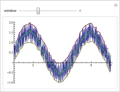
You can also create a moving min (and max) and use BSplineCurve to render a smoothed curve.
These could be made more efficient. They find the min and max over a window.
windowMin[data_, w_][pt_] := {pt,
  Min[Cases[data, {x_, y_} /; pt - w <= x <= pt + w][[All, 2]]]}

windowMax[data_, w_][pt_] := {pt,
  Max[Cases[data, {x_, y_} /; pt - w <= x <= pt + w][[All, 2]]]}
This function plots the original data with the BSplineCurve envelope. The parameter w sets the window width.
f[w_] := With[{data = Transpose[{xaxis, yaxis}]},
  Show[ListLinePlot[data,
    PlotStyle -> Directive[{Blue, Opacity[.2]}]],
   With[{pts = Table[windowMin[data, w][t], {t, 0, 10, w - w/10}]},
    Graphics[{Red, BSplineCurve[pts]}]],
   With[{pts = Table[windowMax[data, w][t], {t, 0, 10, w - w/10}]},
    Graphics[{Red, BSplineCurve[pts]}]]]]
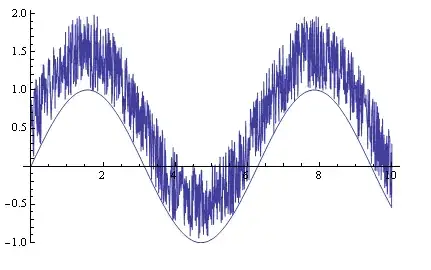
Some examples...
f[.2]

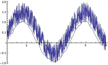
f[.1]

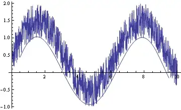
f[.025]

Edit: In response to the comment, here is a more general form of f which allows for a list of xdata and a list of ydata provided they are of equal length. The min and max of the Tables are chosen to be the range of the x data.
f[xdata_, ydata_, w_] /; Length[xdata] == Length[ydata] :=
 Block[{data = Transpose[{xdata, ydata}], xmin = Min[xdata],
   xmax = Max[xdata]},
  Show[ListLinePlot[data,
    PlotStyle -> Directive[{Blue, Opacity[.2]}]],
   With[{pts =
      Table[windowMin[data, w][t], {t, xmin, xmax,
        w - w/(xmax - xmin)}]}, Graphics[{Red, BSplineCurve[pts]}]],
   With[{pts =
      Table[windowMax[data, w][t], {t, xmin, xmax,
        w - w/(xmax - xmin)}]}, Graphics[{Red, BSplineCurve[pts]}]]]]