plotting a trig functions along with its envelope

Question

Note: This questions is quite different from the ones referred to in the comments. Those deal with numerical questions, while this one is algebraic.

I have plots of the following type:

Plot[Cos[50 t] + Cos[51 t], {t, 0, 10}]

enter image description here

I would like to plot a envelope over this plot, i.e. another plot that joins all of maxima and minima of this plot respectively. Here is my attempt, but it's not exactly what I'd like:

Plot[{Cos[50 t] + Cos[51 t], Cos[t] + 1.5, -Cos[t] - 1.5}, {t, 0, 10}]

enter image description here

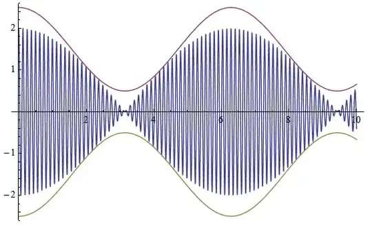
How can I generate the actual envelope?

this is completely true but this is for the Fig.1, I want to access to sheath while I do not access to any formula for that. — Unbelievable, Jun 03 '14 at 18:32
Well, you've got to give us some kind of input to start with. — Mark McClure, Jun 03 '14 at 18:34
I plotted these ones with: Plot[{Cos[50 t] + Cos[51 t], Cos[t] + 1.5, -Cos[t] - 1.5}, {t, 0, 10}], I used of simulated functions 'Cos[t] + 1.5' and '-Cos[t] - 1.5' for the sheath. — Unbelievable, Jun 03 '14 at 18:36
In that case, your sheath is given pretty much perfectly by $\pm 2\cos(t/2)$, but maybe that's not what you want? — Mark McClure, Jun 03 '14 at 18:40
Yes, it was exactly I want. thank you so much. Now, I must think why for every frequency, we can use of the +-2Cos[t/2]. — Unbelievable, Jun 03 '14 at 18:45
Ok. I can understand why for every frequency which are different with the one the frequency of the sheath will be 1/2 and for different equal to 2, sheath frequency will be 1 and so on. — Unbelievable, Jun 03 '14 at 18:56
I edited your question. You should make sure that I preserved your intended meaning. — Mark McClure, Jun 03 '14 at 19:27
Nearly a duplicate of Elegant way of obtaining the envelope of oscillating function, which is a duplicate of Mathematica envelope for the bottom of a plot, a generic function. But this one just straight trigonometry. — Michael E2, Aug 28 '14 at 00:20

score 19 · Answer 1 · edited Apr 13 '17 at 12:55

19

Don't mind me, I'm just having fun.

Grab the definition of HilbertTransform from this previous post, and then:

f[t_] := Cos[50 t] + Cos[51 t] + Sin[53 t] (* more sinusoids = more fun *)
g[t_] := Evaluate@HilbertTransform[f[τ], τ, t]
h[t_] := Abs[f[t] + I g[t]]
Plot[{f[t], h[t], -h[t]}, {t, 0, 10}, ImageSize -> Large, PlotPoints -> 100,
 PlotStyle -> {Automatic, Black, Black}]

enter image description here

You can see that the envelope has a nice analytical form:

ComplexExpand[h[t]] // FullSimplify

$\sqrt{3 + 2\cos t + 2\sin 2t + 2\sin 3t}$

Further reading: analytic representation.

edited Apr 13 '17 at 12:55

Community

1

answered Jun 04 '14 at 03:55

This way though doesn't seem to catch when the envelope should go to zero. Shouldn't it e.g. vanish near 2? – Ruslan Jun 04 '14 at 08:34
1

Should it? It still looks like a sinusoid with small but nonzero amplitude there. (The envelope correctly goes to zero for the original function in the question, if that's what you're concerned about.) – Jun 04 '14 at 08:55
Ah, OK then, you're right. – Ruslan Jun 04 '14 at 09:02
@Rahul: wow! that's really cool! Would this also work on a set of discrete data? Something like ListLinePlot[Accumulate[RandomReal[{-1, 1}, 1000]]] ... If not, how could one modify it so that it does? I have a bunch of data that makes a seemingly random curve like that and I'd like be able to integrate over some area under the curve like the one that you generated.
(Hmmm, i just copy pasted your code, but didn't get the black curve :( what could have gone wrong?)
– Raksha May 16 '15 at 03:46
1

@Solarmew: You first need to copy the definition of the Hilbert transform from the post I linked to. It also gives a discrete version of the transform, which you could use in much the same way on discrete data. – May 16 '15 at 15:58

Mark McClure · Accepted Answer · 2014-06-03T19:19:03.590

15

Playing with the manipulate below might help. It's based on the the acoustics of beats.

Manipulate[Plot[
  {Cos[a*t] + Cos[b*t], 2*Cos[(b - a) t/2], -2*Cos[(b - a) t/2]}, {t, 0, 10},
  PlotStyle -> {
   Directive[Opacity[0.7]], 
   Directive[Black, Thick], 
   Directive[Black, Thick]}],
 {{a, 20}, 1, 50}, {{b, 21}, 1, 50}]

enter image description here

edited Jun 03 '14 at 19:19

answered Jun 03 '14 at 18:56

Mark McClure

32,469
3
103
161

Thank you so much. this is correct – Unbelievable Jun 03 '14 at 18:58

plotting a trig functions along with its envelope

2 Answers2

Linked

Related