How do I draw a Circular Graph colored like this in Mathematica?

Question

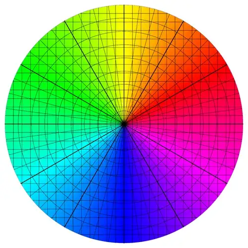
I must plot some data in radians and would like to use this image as a background to that graph. Although it looks good, the lines are degraded in image form; thus, the reason for this question. Can something like this be drawn in Mathematica?

Answer 1

Here's a start. I'll leave the labeling and fine tuning the details to you:

With[{thin = {Thin, Opacity[0.4]}},
    RegionPlot[x^2 + y^2 <= 1, {x, -1, 1}, {y, -1, 1}, 
        ColorFunction -> (Hue[ArcTan[#, #2]/(2 π)] &), 
        ColorFunctionScaling -> False, PlotPoints -> 100, Frame -> False,
        Mesh -> {21, 21, 10, 7, 47}, MeshStyle -> {thin, thin, thin, thin, thin}, 
        MeshFunctions -> {# &, #2 &, Norm[{#1, #2}] &, ArcTan[# , #2] &, ArcTan[# , #2] &}
    ]
]

Answer 2

It is of course possible to draw everything manually.

Manipulate[
 With[{
   colArea = 
    Polygon[#2, VertexColors -> ConstantArray[Hue[#1/(2 Pi)], 3]] & @@@ 
    Table[{phi, {{0, 0}, {Cos[phi], Sin[phi]}, {Cos[phi + 2 Pi/colors], 
       Sin[phi + 2 Pi/colors]}}}, {phi, 0, 2 Pi - 2 Pi/colors, 2 Pi/colors}],
   gridLines = 
    Table[{{x, -#}, {x, #}} &[Sqrt[1 - x^2]], {x, -1, 1, 
      2/(grid - 1)}],
   radLines = Table[{{0, 0}, {Cos[phi], Sin[phi]}}, 
      {phi, 0, 2 Pi - 2 Pi/radiants, 2 Pi/radiants}],
   cirLines = With[{
     circle = Table[{Cos[phi], Sin[phi]}, {phi, 0, 2 Pi, Pi/20}]},
     Table[r*circle, {r, 0, 1, 1/circles}]
   ]},
   Graphics[{
    colArea, Black, Thin, Line[gridLines], 
    Line[Map[Reverse, gridLines, {2}]], Darker@Gray, Line@radLines, 
    Line /@ cirLines}]],
 {circles, 3, 10, 1},
 {radiants, 4, 20, 1},
 {grid, 5, 20, 1},
 {{colors, 20}, 4, 120, 1}
 ]

Update

By the way, it is not required to create a new coordinate list for all graphics primitives. This was only done to make the code verbose enough. The color disk, the radial lines and the circles can all be created easily using the same underlying data. Here the Span operator (;;) becomes handy, to achieve high resolution in the color disk, but have only some radial grid lines.

With[{pts = Append[#, First[#]] &@ Table[{r {Cos[phi], Sin[phi]}, phi/(2 Pi)}, 
  {phi, 0, 2 Pi, .1}, {r, 0, 1, .1}]},
Graphics[{Polygon[{{0, 0}, First[#1], First[#2]}, 
  VertexColors -> (Hue /@ {{0, 0, 1}, Last[#1], Last[#2]})] & @@@ 
    Partition[pts[[All, -1, {1, 2}]], 2, 1],
  Black, Opacity[.5], Line[pts[[;; ;; 3, All, 1]]], Line[Transpose[pts[[All, All, 1]]]],
  Opacity[.2], {Line[#], Line[Map[Reverse, #, {2}]]} &@
    Table[{{x, #}, {x, -#}} &@Sqrt[1 - x^2], {x, -1, 1, .1}]
  }]]

Answer 3

Just for fun, only the color wheel drawing part done with Disk sectors:

With[{sectors = 360},
 angle = 2 Pi/sectors;
 Graphics[
  Table[{Hue[i/sectors], EdgeForm[{Thick, Hue[i/sectors]}],  
    Disk[{0, 0}, 1, {i angle, (i + 1) angle}]}, {i, 0, sectors - 1}]]]

I had to use a thick EdgeForm because without it I was getting a moiré pattern in the rendering.

Answer 4

I set out to do this differently from R.M, but I ended up with something very similar. Nevertheless, I think there is a certain simplicity that results from my using ParametricPlot, so here it is:

ParametricPlot[
 r {Cos[t], Sin[t]}, {t, 0, 2 Pi}, {r, 0, 1},
 Axes -> False, Frame -> False,
 Mesh -> {47, 11, {0}, 8, 27, 27},
 MeshFunctions -> {#3 &, #3 &, #3 &, #4 &, # &, #2 &},
 MeshStyle -> ({#, #2, #2, #, #, #} &[Opacity[0.5], Thick]),
 ColorFunction -> (Hue[#3 - 1/12] &)
]

A complication that arose with this method is that I needed to specifically add the line at zero (that is, east), as I could not get Mesh to do this automatically.

Answer 5

Here is another method based on RegionPlot[], similar to rm's solution. There are a few wrinkles in this version, however:

1. I use PolarPlot[] to generate the ticks for me. (I know about the hidden functions behind the generation of the polar ticks, but I couldn't figure how to use them directly.)

2. I use the saturation and brightness arguments of Hue[] to generate the meshes as part of the color function. The idea was stolen adapted from the solutions of Heike and Simon in this answer, but I did change a few things around.

Now, on to the routine:

hueWithMesh[x_, y_, hx_: 1/10, hr_: 1/8, ht_: 1/24, r1_: 2/5, r2_: 1/2, g_: 1/5] := 
  Block[{ph = Arg[x + I y]/π, s, b}, 
        s = r1 + (1 - r1) Abs[(Mod[2 Abs[x + I y]/hr, 2, 1] - 2) (Mod[ph/ht, 2, 1] - 2)]^g;
        b = r2 + (1 - r2) Abs[(Mod[2 x/hx, 2, 1] - 2) (Mod[2 y/hx, 2, 1] - 2)]^g;
        Hue[ph/2 - 1/12, s, Max[1 - s^2, b]]]

 Show[PolarPlot[1/Sqrt[2], {t, -π, π}, MaxRecursion -> 0, PlotPoints -> 6,
                PlotRange -> 1, PlotStyle -> None, PolarAxes -> Automatic], 
      RegionPlot[Abs[x + I y] <= 1, {x, -1, 1}, {y, -1, 1}, BoundaryStyle -> None, 
                 ColorFunction -> (hueWithMesh[#1, #2] &), ColorFunctionScaling -> False, 
                 Frame -> False, PlotPoints -> 200], PlotRange -> All]

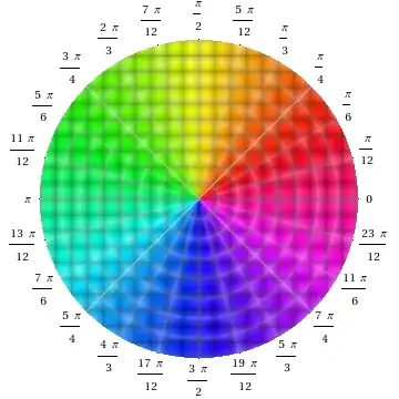
As you might notice from the implementation of hueWithMesh[], the parameters hr, ht, and hx all control the spacing in the rectangular and polar meshes, while r1, r2, and g all control the saturation/brightness for the meshes. You can tweak these parameters to your taste.

Answer 6

Since you've already gotten a bunch of fine answers, I'll just quietly post this variation:

DensityPlot[ArcTan[x, y], {x, -1, 1}, {y, -1, 1}, 
            ColorFunction -> (Hue[# - 7/12] &), Frame -> False, Mesh -> {30, 30, 8, 49}, 
            MeshFunctions -> {#1 &, #2 &, Abs[#1 + I #2] &, Arg[#1 + I #2] &}, 
            MeshStyle -> {Opacity[1/3, GrayLevel[1/5]], Opacity[1/3, GrayLevel[1/5]],
                          Opacity[1/3, GrayLevel[1/2]], Opacity[1/3, GrayLevel[1/2]]},
            PlotPoints -> 45, RegionFunction -> (Norm[{#1, #2}] < 1 &)]

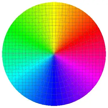
Tick addition is left for as an exercise for less lazy readers.

Answer 7

Using Polygon:

With[{d = 2 Pi/360}, 
 Graphics[Table[{Hue[t/( 2 Pi)], EdgeForm@Hue[t/( 2 Pi)], 
    Polygon@{{0, 0}, {Cos[t], Sin[t]}, {Cos[t + d], Sin[t + d]}}}, {t, d, 2 Pi, d}]]
 ]