I solved it!
The issue was that BC must be $\pm \infty$ and the correct normalization needed to be used. Similar to what was done for your generalized wave pde question Difficulty to Solve the Generalized Wave Equation
The analytical solution to the general heat pde in 1D
\begin{align*}
u_{t}+\frac{v}{2}x^{2}u & =\frac{v}{2}u_{xx}\\
u\left( x,0\right) & =f\left( x\right) =e^{-\frac{x^{2}}{2}}H_{1}\left(
x\right) +\frac{1}{5}e^{-\frac{x^{2}}{2}}H_{4}\left( x\right) +\frac
{1}{100}e^{-\frac{x^{2}}{2}}H_{6}\left( x\right) \\
u\left( -\infty,t\right) & =0\\
u\left( +\infty,t\right) & =0
\end{align*}
is the following
$$
u(x,t)=e^{-\frac{x^{2}}{2}}\left( e^{-\frac{v}{2}3t}H_{1}\left( x\right)
+\frac{1}{5}e^{-\frac{v}{2}9t}H_{4}\left( x\right) +\frac{1}{100}%
e^{-\frac{v}{2}13t}H_{6}\left( x\right) \right)
$$
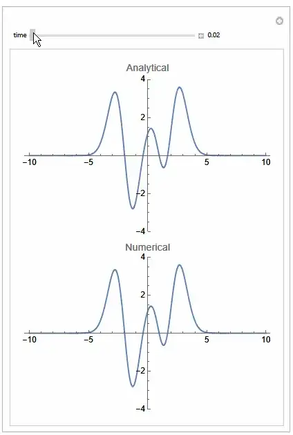
Animation
Code for the above
ClearAll[x, t];
v = 1;
sol[x_, t_] := Exp[-x^2/2]*(Exp[-v/2*3*t]*HermiteH[1, x] +
   1/5*Exp[-v/2*9*t]*HermiteH[4, x] + 1/100*Exp[-v/2*13*t]*HermiteH[6, x])
Y[n_] := Exp[-x^2/2]HermiteH[n, x]
ic    = u[x, 0] == Y[1] + 0.2 Y[4] + 0.01 Y[6]
pde   = D[u[x, t], t] + v/2x^2u[x, t] == v/2D[u[x, t], {x, 2}];
L     = 10; (for NDSolve only)
bc    = {u[-L, t] == 0, u[L, t] == 0}
nsol  = NDSolveValue[{pde, ic, bc}, u, {x, -L, L}, {t, 0, 3}];
Manipulate[
 Grid[{{Plot[sol[x0, t0], {x0, -10, 10}, PerformanceGoal -> "Quality",
      PlotRange -> {Automatic, {-4, 4}}, ImageSize -> 300,
     PlotLabel -> "Analytical"]},
   {Plot[Evaluate[nsol[x0, t0]], {x0, -10, 10},
     PerformanceGoal -> "Quality", PlotRange -> {Automatic, {-4, 4}},
     ImageSize -> 300, PlotLabel -> "Numerical"]
    }}],
 {{t0, 0, "time"}, 0, 3, .01, Appearance -> "Labeled",
  ContinuousAction -> True}, TrackedSymbols :> {t0}]
Hand solution
\begin{align*}
u_{t}+\frac{v}{2}x^{2}u & =\frac{v}{2}u_{xx}\\
u\left( x,0\right) & =f\left( x\right) =e^{-\frac{x^{2}}{2}}H_{1}\left(
x\right) +\frac{1}{5}e^{-\frac{x^{2}}{2}}H_{4}\left( x\right) +\frac
{1}{100}e^{-\frac{x^{2}}{2}}H_{6}\left( x\right) \\
u\left( -\infty,t\right) & =0\\
u\left( +\infty,t\right) & =0
\end{align*}
Let $u=X\left( x\right) T\left( t\right) $, then the pde becomes
\begin{align*}
T^{\prime}X+\frac{v}{2}x^{2}XT & =\frac{v}{2}X^{\prime\prime}T\\
\frac{T^{\prime}}{T}+\frac{v}{2}x^{2} & =\frac{v}{2}\frac{X^{\prime\prime}%
}{X}\\
\frac{2}{v}\frac{T^{\prime}}{T} & =\frac{X^{\prime\prime}}{X}-x^{2}%
\end{align*}
Hence
\begin{align*}
\frac{2}{v}\frac{T^{\prime}}{T} & =-\lambda\\
T^{\prime}+\frac{v}{2}\lambda T & =0
\end{align*}
The solution to the above is
$$
T=Ae^{-\frac{v}{2}\lambda t}%
$$
And
\begin{align*}
\frac{X^{\prime\prime}}{X}-x^{2} & =-\lambda\\
-X^{\prime\prime}+x^{2}X & =\lambda X\\
X\left( -\infty\right) & =0\\
X\left( \infty\right) & =0
\end{align*}
The eigenvalues are (see below) $\lambda_{n}=1+2n$ for $n=0,1,2,3,\cdots$.
Hence $\lambda_{n}=\left\{ 1,3,5,7,\cdots\right\} $ and corresponding
eigenfunction are
\begin{align*}
X_{n} & =e^{-\frac{x^{2}}{2}}H_{n}\left( x\right) \qquad n=0,1,2,3\cdots\\
\lambda_{n} & =\left\{ 1,3,5,7,\cdots\right\}
\end{align*}
Hence the pde solution is linear combination of the solutions $X_{n}T_{n}$ or
\begin{align}
u & =\sum_{n=0}^{\infty}T_{n}X_{n}\tag{1}\\
& =\sum_{n=0}^{\infty}A_{n}e^{-\frac{v}{2}\lambda_{n}t}e^{-\frac{x^{2}}{2}%
}H_{n}\left( x\right) \nonumber
\end{align}
At $t=0$ the above becomes, since $u\left( x,0\right) =f\left( x\right)
=e^{-\frac{x^{2}}{2}}H_{1}\left( x\right) +\frac{1}{5}e^{-\frac{x^{2}}{2}%
}H_{4}\left( x\right) +\frac{1}{100}e^{-\frac{x^{2}}{2}}H_{6}\left(
x\right) $%
\begin{align*}
e^{-\frac{x^{2}}{2}}H_{1}\left( x\right) +\frac{1}{5}e^{-\frac{x^{2}}{2}%
}H_{4}\left( x\right) +\frac{1}{100}e^{-\frac{x^{2}}{2}}H_{6}\left(
x\right) & =\sum_{n=0}^{\infty}A_{n}e^{-\frac{x^{2}}{2}}H_{n}\left(
x\right) \\
e^{-\frac{x^{2}}{2}}\left( H_{1}\left( x\right) +\frac{1}{5}H_{4}\left(
x\right) +\frac{1}{100}H_{6}\left( x\right) \right) & =\sum
_{n=0}^{\infty}A_{n}e^{-\frac{x^{2}}{2}}H_{n}\left( x\right) \\
e^{-x^{2}}\left( H_{1}\left( x\right) +\frac{1}{5}H_{4}\left( x\right)
+\frac{1}{100}H_{6}\left( x\right) \right) & =\sum_{n=0}^{\infty}
A_{n}e^{-x^{2}}H_{n}\left( x\right)
\end{align*}
multiplying both sides by arbitrary $H_{m}\left( x\right) $
$$
e^{-x^{2}}H_{m}\left( x\right) \left( H_{1}\left( x\right) +\frac{1}%
{5}H_{4}\left( x\right) +\frac{1}{100}H_{6}\left( x\right) \right)
=\sum_{n=0}^{\infty}A_{n}e^{-x^{2}}H_{n}\left( x\right) H_{m}\left(
x\right)
$$
Integrating, and moving the integral into the sum on the RHS gives
$$
\int_{-\infty}^{\infty}e^{-x^{2}}H_{m}\left( x\right) H_{1}\left( x\right)
dx+\frac{1}{5}\int_{-\infty}^{\infty}e^{-x^{2}}H_{m}\left( x\right)
H_{4}\left( x\right) dx+\frac{1}{100}\int_{-\infty}^{\infty}e^{-x^{2}}%
H_{m}\left( x\right) H_{6}\left( x\right) dx=\sum_{n=0}^{\infty}A_{n}%
\int_{-\infty}^{\infty}e^{-x^{2}}H_{n}\left( x\right) H_{m}\left( x\right)
dx
$$
By orthogonality $\int_{-\infty}^{\infty}e^{-x^{2}}H_{n}\left( x\right)
H_{m}\left( x\right) dx=\sqrt{\pi}2^{m}m!\delta_{nm}$ (see Wikipedia) hence the above becomes
\begin{align*}
\int_{-\infty}^{\infty}e^{-x^{2}}H_{m}\left( x\right) H_{1}\left( x\right)
dx+\frac{1}{5}\int_{-\infty}^{\infty}e^{-x^{2}}H_{m}\left( x\right)
H_{4}\left( x\right) dx+\frac{1}{100}\int_{-\infty}^{\infty}e^{-x^{2}}%
H_{m}\left( x\right) H_{6}\left( x\right) dx & =A_{m}\sqrt{\pi}2^{m}m!\\
\sqrt{\pi}2\delta_{n,1}+\frac{1}{5}\left( \sqrt{\pi}2^{4}4!\right)
\delta_{n,4}+\frac{1}{100}\left( \sqrt{\pi}2^{6}6!\right) \delta_{n,6} &
=A_{n}\sqrt{\pi}2^{n}n!
\end{align*}
Hence
\begin{align*}
A_{n} & =\frac{1}{\sqrt{\pi}2^{n}n!}\left( \sqrt{\pi}2\delta_{n,1}+\frac
{1}{5}\left( \sqrt{\pi}2^{4}4!\right) \delta_{n,4}+\frac{1}{100}\left(
\sqrt{\pi}2^{6}6!\right) \delta_{n,6}\right)
\end{align*}
Therefore the solution (1) becomes
\begin{align}
u\left( x,t\right) & =\sum_{n=0}^{\infty}A_{n}e^{-\frac{v}{2}\left(
2n+1\right) t}e^{-\frac{x^{2}}{2}}H_{n}\left( x\right) \tag{2}\\
& =A_{1}e^{-\frac{v}{2}\left( 2+1\right) t}e^{-\frac{x^{2}}{2}}H_{1}\left(
x\right) +A_{4}e^{-\frac{v}{2}\left( 8+1\right) t}e^{-\frac{x^{2}}{2}}
H_{4}\left( x\right) +A_{6}e^{-\frac{v}{2}\left( 12+1\right) t}
e^{-\frac{x^{2}}{2}}H_{6}\left( x\right) \\
& =e^{-\frac{v}{2}3t}e^{-\frac{x^{2}}{2}}H_{1}\left( x\right) +\frac{1}
{5}e^{-\frac{v}{2}9t}e^{-\frac{x^{2}}{2}}H_{4}\left( x\right) +\frac{1}
{100}e^{-\frac{v}{2}13t}e^{-\frac{x^{2}}{2}}H_{6}\left( x\right)
\end{align}
Therefore
$$
\boxed{
u(x,t)=e^{-\frac{x^{2}}{2}}\left( e^{-\frac{v}{2}3t}H_{1}\left( x\right)
+\frac{1}{5}e^{-\frac{v}{2}9t}H_{4}\left( x\right) +\frac{1}{100}
e^{-\frac{v}{2}13t}H_{6}\left( x\right) \right)
}
$$
Attempt with DSolve
ClearAll[x, t, n];
Y[n_] := Exp[-x^2/2]*HermiteH[n, x]
v = 1;
ic = u[x, 0] == Y[1] + 0.2 Y[4] + 0.01 Y[6]
pde = D[u[x, t], t] + v/2*x^2*u[x, t] == v/2*D[u[x, t], {x, 2}];
bc = {u[-Infinity, t] == 0, u[Infinity, t] == 0}
sol = DSolve[{pde, ic, bc}, u[x, t], {x, t}]
No solution.
 Update


DEigensystemonX[x]ode and you will see that it can't solve it. – Nasser Mar 20 '23 at 23:07DSolvedoesn't seem to be able to handle the problem directly. – xzczd Mar 21 '23 at 11:18