You can try "shooting method":
eqn1 = t x'[t] - (-x[t] + y[t]);
eqn2 = t y'[t] - (-5 t^2/x[t]^2 + x[t] - y[t]);
sol = NDSolve[{eqn1 == 0, eqn2 == 0, x[0] == y[0], x[1] == 1}, {x, y}, {t, 0, 1},
              Method -> {"Shooting", "StartingInitialConditions" ->
                                     {x[1] == 1, y[1] == 2/100 + 91/16000}}];
Plot[{x[t], y[t]} /. sol, {t, 0, 1}, Evaluated -> True]
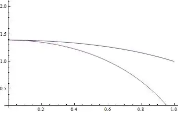
The "StartingInitialConditions" above is found by trial and error, despite some warnings generated, the solution is reliable enough:
(* Error check *)
Plot[{eqn1, eqn2} /. sol, {t, 0, 1}, Evaluated -> True]
Plot[{eqn1, eqn2} /. sol, {t, 0, 1}, PlotRange -> All]


Edit
Let me add some explanations about how I found a good initial condition. As I've mentioned in the comment below, what I used is just method of exhaustion… yeah, exhaustion, sounds clumsy but it's really powerful.
First, I define the following function for the realization of the method:
ClearAll[try]
SetAttributes[try, Listable]
try[i_] :=(* try[i] = *){i, Quiet@NDSolve[{eqn1 == 0, eqn2 == 0, x[0] == y[0], x[1] == 1},
                           {x, y}, {t, 0, 1}, Method -> {"Shooting",
                           "StartingInitialConditions" -> {x[1] == 1, y[1] == i}}]};
If you add the try[i] = in the note into the code, Mathematica will remember all the calculated try[i] so repetitive computation can be avoided when rechecking, of course this will consume more memory and not that necessary for your case.
We don't know what value will be a proper initial condition, but it's not that hard to guess the approximate extent of it, based on some observations to the equations and boundary conditions, I guess that y[1] may be between -10 and 10. So I tried:
midpoint = 0; step = 1;
try@Range[midpoint - 10 step, midpoint + 10 step, step] // MatrixForm

All of the trials fail in the middle of the domain of t, but one of them stick out to about 0.02, with y[1] == 0, which means a proper initial condition may be near 0, so I go on trying:
midpoint = 0; step = 1/10;
try@Range[midpoint - 9 step, midpoint + 9 step, step] // MatrixForm

The best condition we found is still y[1] == 0 but the scope is smaller now… wait, so far I was modifying midpoint and step by hand, why not make them modified automatically?:
Clear[leftboundary, area]
(* leftboundary is used for the extraction
   of the left boundary of the interpolating function,
   it's specifically designed for the structure of try[i]. *)
leftboundary = First@First@First@First[x /. Last@#] &;
(* area is used for the generation of possible y[1] *)
area[midpoint_, step_] := Range[midpoint - 9 step, midpoint + 9 step, step]

NestWhile[{First@SortBy[try@area[First@#, #2], leftboundary], #2/10} & @@ # &,
          {try[0], 1/100}, leftboundary@First@# > 10^-16 &]
{513/20000, 1.24278*10^-128, 1/1000000}
OK, this time we get a even better initial condition: y[1] == 513/20000.
TableandNest, for this part I can add something to my answer tomorrow, but now I'd like to go to bed. :D – xzczd Jul 17 '13 at 15:15nestwhile,{First@SortBy[f@h[First@#[[1]], #[[2]]], g], #[[2]]/10} &acts on{f[0], 1/100}, which meansf@h[First@#[[1]], #[[2]]], g]acts onf[0], and#[[2]]/10acts on1/100, I am confused. could you explain it more clearly? – 3c. Oct 20 '13 at 23:28NestWhile, for the first round of iteration,#in the first argument means the second argument ofNestWhilei.e.#[[1]]represents{f[0], 1/100}[[1]],#[[2]]represents{f[0], 1/100}[[2]]so the calculated expression is{First@SortBy[f@h[First@f[0], 1/100], g], 1/100/10}. – xzczd Oct 21 '13 at 05:09i=0, what if you do not know that, can you start from anyiand find the right initial value? – 3c. Oct 21 '13 at 19:23iso far… But also notice that the rough range for the current algorithm can be quite extensive. (What I used is $[-10, 10]$ at beginning.) – xzczd Oct 22 '13 at 02:310, I need to find the initial conditioni. I have no idea to figure it out – 3c. Oct 22 '13 at 14:44