Combination of a Contourplot and a Graphics Object

Question

I want to combine the following to graphs.

cartPoints = Table[With[{x = RandomReal[]}, {1/(2*Pi), ArcCos[x]}], {10}];
Graphics[Arrow[{{0, 0}, #}] & /@ CoordinateTransform["Polar" -> "Cartesian", cartPoints], 
Frame -> True, FrameTicks -> None, AspectRatio -> 1, 
PlotRange -> {{0, 1/(2*Pi)}, {0, 1/(2*Pi)}}, 
FrameLabel -> {{"z", ""}, {"y", ""}}, 
LabelStyle -> { FontFamily -> "Arial", FontSize -> 14}, 
BaseStyle -> {FontFamily -> "Arial", FontSize -> 14}]

ContourPlot[Cos[x^2 + y^2], {x, -Sqrt[Pi]/2, Sqrt[Pi]/2}, {y, -Sqrt[Pi]/2, 
Sqrt[Pi]/2}, FrameLabel -> {{"x", ""}, {"y", ""}}, 
LabelStyle -> { FontFamily -> "Arial", FontSize -> 14}, 
BaseStyle -> {FontFamily -> "Arial", FontSize -> 14}]

How can I arrange both graphs in 3D? The Countourplot should be the bottom of the resultung graph and the arrows should point in z direction

Yes, I want to combine both graphs in a 3D Plot. Do I have to use a Graphics3D Plot for the arrow Plot to do so? — user8905, Aug 06 '13 at 09:55
Some possible duplicates: 3665, 7772, 19870. @user8905 Please check and see if any of these answer your question. — Michael E2, Aug 06 '13 at 10:49

score 1 · Answer 1 · answered Aug 06 '13 at 16:52

I don't know what your ultimate objective is here and what the arrows are to represent. Since no one has given a specific answer yet I'm going to do it using the Presentations Application, which I sell. First I'm going to change your arrow data so there are more or less evenly spaced angles between the arrows and the xy-plane. I decided to draw the arrows directly in 3D. (Maybe they should also be randomly rotated around the z axis?)

polarPoints = Table[{1/2, RandomReal[{0, \[Pi]/2}]}, {5}];
cartesianPoints = 
  CoordinateTransform["Polar" -> "Cartesian", 
    polarPoints] /. {x_, z_} -> {x, 0, z};

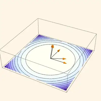
Then here is a plot with the contour drawing in the z = 0 plane and the arrows at the origin. RaiseTo3D[0&] raises the 2D ContourDraw graphics to the zero plane. Then we draw the arrows directly in 3D. NeutralLighting is similar to Lighting -> Neutral but with much more control. We want neutral lighting to preserve the colors of the contour plot.

<< Presentations`

Draw3DItems[
 {ContourDraw[
    Cos[x^2 + y^2], {x, -Sqrt[Pi]/2, Sqrt[Pi]/2}, {y, -Sqrt[Pi]/2, 
     Sqrt[Pi]/2}] // RaiseTo3D[0 &],
  Orange, ,
  Arrowheads[0.05],
  Arrow[Tube[{{0, 0, 0}, #}]] & /@ cartesianPoints},
 NiceRotation,
 NeutralLighting[0, 0.3, 0.5],
 PlotRange -> {-0.01, 0.55},
 BoxRatios -> Automatic,
 ImageSize -> 400]

enter image description here

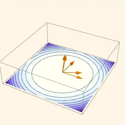
Presentations also has a legacy Arrow3D function, which predated the Mathematica function, and has a few different features. For example it is easier to separately control the directives for the shaft and arrowheads.

Draw3DItems[
 {ContourDraw[
    Cos[x^2 + y^2], {x, -Sqrt[Pi]/2, Sqrt[Pi]/2}, {y, -Sqrt[Pi]/2, 
     Sqrt[Pi]/2}] // RaiseTo3D[0 &],
  Arrow3D[{0, 0, 0}, #, {0.1, 0.5, 20, "Absolute", 
      PlotStyle -> {Orange}}, {AbsoluteThickness[1], Black}] & /@ 
   cartesianPoints},
 NiceRotation,
 NeutralLighting[0, 0.3, 0.5],
 PlotRange -> {-0.01, 0.55},
 Axes -> False,
 BoxRatios -> Automatic,
 ImageSize -> 400]

enter image description here

Combination of a Contourplot and a Graphics Object

1 Answers1