Note: This question is for those chaotic systems where the order of maximal Lyapunov exponent is around $10^{-3}$. So it's different from normal chaotic systems like Hénon–Heiles system, Yang-Mills-Higgs System, Double Pendulum or the famous Lorenz Attractor.
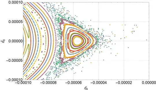
The related problem: I am trying to reproduce my results for the Poincaré section published here (Specifically one of the sub-figures in Figure $8$ on page $15$ given below), which I plotted by making use of an algorithm developed by @Alex Trounev. I am trying to plot the same this time by a different interactive algorithm of @E. Chan-López.
The code being used is as follows:
lagrangian = (8 x[t]^2)/3 + (4 x[t]^3)/3 - 6 y[t]^2 +
   148/7 x[t] y[t]^2 + Derivative[1][x][t]^2 +
   1/3 y[t] Derivative[1][x][t] Derivative[1][y][t] +
   Derivative[1][y][t]^2 + 1/5  x[t]  Derivative[1][y][t]^2;
Px = D[lagrangian, x'[t]];
Py = D[lagrangian, y'[t]];
hamiltonian = ((Px x'[t] + Py y'[t]) -
      lagrangian) /. (Solve[{px[t] == Px, py[t] == Py}, {x'[t],
        y'[t]}] // Last) // FullSimplify;
{a1, b1, c1, d1} = {D[hamiltonian, px[t]],
  D[hamiltonian,
   py[t]], -D[hamiltonian, x[t]], -D[hamiltonian,
    y[t]]}; hameqns = {x'[t] == a1, px'[t] == c1, y'[t] == b1,
  py'[t] == d1};
constraint =
 FullSimplify[
  Last[(py0 /.
     Solve[e == (hamiltonian /. {x[t] -> x0, px[t] -> px0, y[t] -> 0,
          py[t] -> py0}), py0])]]
PoincareSections[{x0_, px0_, y0_, py0_}, e_, tmax_] :=
 Block[{constraint, x, px, y, py},
  constraint = (
   I Sqrt[5 + x0] Sqrt[-12 e + 3 px0^2 - 16 x0^2 (2 + x0)])/Sqrt[15];
  If[Head[N[constraint]] === Complex, Nothing,
   If[# == {}, {}, First[#]] &@
    Last[Reap[
      NDSolve[{hameqns, x[0] == x0, px[0] == px0, y[0] == y0,
        py[0] == constraint,
        WhenEvent[y[t],
         Sow[{x[t], px[t]}, "LocationMethod" -> "EvenLocator"]]}, {x,
        px, y, py}, {t, 0, tmax}, MaxSteps -> ∞,
       MaxStepSize -> 0.1]]]]]
style = {PlotStyle -> {{AbsolutePointSize[1], Opacity[0.4]}},
   AspectRatio -> 1, ImageSize -> 420, PlotHighlighting -> None};
DynamicModule[{f = {}},
 Column[{Dynamic[
    MatrixForm@{MousePosition["Graphics", "Mouse not in graphics!"]}],
    Row[{ClickPane[
      Dynamic@ListPlot[f,
        style], (AppendTo[f,
         PoincareSections[{#[[1]], #[[2]], 0, 0}, 10^-5, 3000]]) &],
     Button[Style["Copy orbit list", 12],
      CopyToClipboard[Iconize[f, "Orbit list"]],
      ImageSize -> Automatic, Alignment -> Center,
      Appearance -> {"Palette", "Pressed"}]}, "  "]},
  Alignment -> Center]]
Now, the above algorithm doesn't work simply because the Head of the constraint turns out to be complex. But if we calculate it, technically, it's not a complex number. A simple example can explain the reason:
The issue:
a = N[constraint] /. x0 -> -1/1000 /. px0 -> 1/1000 /. e -> 10^-5
(-0.007046375030231264+0. I)
Head[a]
(Complex)
The number is Real, but the Head turns out to be Complex only because it is in the form of a+Ib.
If I comment out the condition If[Head[N[constraint]] === Complex in the code, it works, but the system hangs after 3 or 4 mouse clicks. How to rectify this issue?
Edit: Issue resolved Thanks to @BobHanlon, the issue is solved.
    PoincareSections[{x0_, px0_, y0_, py0_}, e_, tmax_] :=
     Block[{constraint, x, px, y, py},
      constraint =
       N[(I   Sqrt[
             5 + x0]   Sqrt[-12   e + 3   px0^2 - 16   x0^2   (2 + x0)])/
          Sqrt[15]] // Chop;
      If[Head[N[constraint]] === Complex, Nothing,
       If[# == {}, {}, First[#]] &@
        Last[Reap[
          NDSolve[{hameqns, x[0] == x0, px[0] == px0, y[0] == y0,
            py[0] == constraint,
            WhenEvent[y[t],
             Sow[{x[t], px[t]}, "LocationMethod" -> "EvenLocator"]]}, {x,
            px, y, py}, {t, 0, tmax}, MaxSteps -> ∞,
           MaxStepSize -> 0.1]]]]]
style = {PlotStyle -> {{PointSize[.005], Opacity[0.9]}},
   AspectRatio -> 1, ImageSize -> 420,
   PlotHighlighting -> None};
DynamicModule[{f = {}},
 Column[{Dynamic[
    MatrixForm@{MousePosition["Graphics", "Mouse not in graphics!"]}],
    Row[{ClickPane[
      Dynamic@ListPlot[f,
        style], (AppendTo[f,
         PoincareSections[{#[[1]], #[[2]], 0, 0}, 10^-5, 3000]]) &],
     Button[Style["Copy orbit list", 12],
      CopyToClipboard[Iconize[f, "Orbit list"]],
      ImageSize -> Automatic, Alignment -> Center,
      Appearance -> {"Palette", "Pressed"}]}, "  "]},
  Alignment -> Center]]
Choosing the best NDSolve Method
Rectified code used for a close up:
par = {9.07, 11.73, 5.80, 2.18, 4.36, -2.645, 6.023}; {K1, K2, K3, K4,
   K5, ωsq[0], ωsq[1]} = Rationalize[par, 10^-30];
lagrangianold =
  Sum[c[n]'[t]^2 - c[n][t]^2  ωsq[n], {n, {0, 1}}] +
   K1  c[0][t]^3 + K2  c[0][t]  c[1][t]^2 + K3  c[0][t]  c[0]'[t]^2 +
   K4  c[0][t]  c[1]'[t]^2 + K5  c[0]'[t]  c[1][t]  c[1]'[t];
c[0][t_] :=
  OverTilde[c][0][t] + α1*OverTilde[c][0][t]^2 + α2*
    OverTilde[c][1][t]^2;
c[1][t_] :=
  OverTilde[c][1][t] + α3*OverTilde[c][0][t]*OverTilde[c][1][t];
α1 = -29/20; α2 = -1/2; α3 = -1;
n = Expand[lagrangianold];
vars = {OverTilde[c][0][t], OverTilde[c][1][t],
   Derivative[1][OverTilde[c][0]][t],
   Derivative[1][OverTilde[c][1]][t]};
lagrangianew =
  Normal[Series[n /. Thread[vars -> m*vars], {m, 0, 3}]] /. m -> 1;
    lagrangian =
  Simplify[
   lagrangianew /. OverTilde[c][0] -> x /. OverTilde[c][1] -> y];
Px = D[lagrangian, x'[t]];
Py = D[lagrangian, y'[t]];
hamiltonian = ((Px x'[t] + Py y'[t]) -
      lagrangian) /. (Solve[{px[t] == Px, py[t] == Py}, {x'[t],
        y'[t]}] // Last) // FullSimplify;
{a1, b1, c1, d1} = {D[hamiltonian, px[t]],
  D[hamiltonian,
   py[t]], -D[hamiltonian, x[t]], -D[hamiltonian,
    y[t]]}; hameqns = {x'[t] == a1, px'[t] == c1, y'[t] == b1,
  py'[t] == d1};
constraint =
 FullSimplify[
  Last[(py0 /.
     Solve[e == (hamiltonian /. {x[t] -> x0, px[t] -> px0, y[t] -> 0,
          py[t] -> py0}), py0])]]
PoincareSections[{x0_, px0_, y0_, py0_}, e_, tmax_] :=
 Block[{constraint, x, px, y, py},
  constraint =
   Chop[N[1/50  Sqrt[-5 - (9 x0)/10]
        Sqrt[-2000 e + 500 px0^2 - x0^2 (5290 + 2799 x0)]]];
  If[Head[N[constraint]] === Complex, Nothing,
   If[# == {}, {}, First[#]] &@
    Last[Reap[
      NDSolve[{hameqns, x[0] == x0, px[0] == px0, y[0] == y0,
        py[0] == constraint,
        WhenEvent[y[t],
         Sow[{x[t], px[t]}, "LocationMethod" -> "EvenLocator"]]}, {x,
        px, y, py}, {t, 0, tmax}, MaxSteps -> ∞,
       MaxStepSize -> 0.1, Method -> "StiffnessSwitching"]]]]]
style = {PlotStyle -> {{PointSize[.005], Opacity[0.9]}},
   AspectRatio -> 1, ImageSize -> 300,
   PlotRange -> {{-0.0001, 0}, {-0.0001, 0.0001}},
   PlotHighlighting -> None};
Off[NDSolve::ndsz]
DynamicModule[{f = {}},
 Column[{Dynamic[
    MatrixForm@{MousePosition["Graphics", "Mouse not in graphics!"]}],
    Row[{ClickPane[
      Dynamic@ListPlot[f,
        style], (AppendTo[f,
         PoincareSections[{#[[1]], #[[2]], 0, 0}, 10^-5, 2000]]) &],
     Button[Style["Copy orbit list", 12],
      CopyToClipboard[Iconize[f, "Orbit list"]],
      ImageSize -> Automatic, Alignment -> Center,
      Appearance -> {"Palette", "Pressed"}]}, "  "]},
  Alignment -> Center]]
I have one minor problem now for a close-up of the above section:
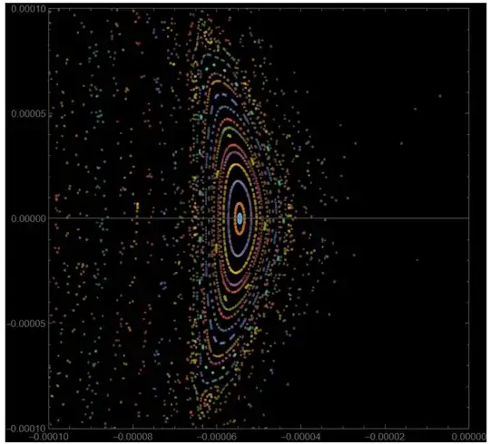
I get an NDSolve warning message, which I turn off. Still, the plot I get differs from the original when I use Method -> "ImplicitRungeKutta" instead of Automatic or some other like "StiffnessSwitching".
Here is a result found using two different methods for comparison:
Why is it that the results are scaled in the y-axis, and which method should be considered the best in such a case? The methods that I used are also not easily seen in the documentation. Also, any help in making the code more elegant(like avoiding warnings) would be genuinely beneficial!


PoincareSectionschange the definition ofconstraintto readconstraint = N[(I Sqrt[5 + x0] Sqrt[-12 e + 3 px0^2 - 16 x0^2 (2 + x0)])/ Sqrt[15]] // Chop;TheChopwill remove imaginary artifacts. – Bob Hanlon Mar 05 '24 at 05:25ImplicitRungeKuttawithImplicitRungeKuttaGaussCoefficientswhich is also symplectic. Projection method can be usefull too – I.M. Mar 06 '24 at 06:19Optionssection ofNDSolvebut hidden inside theTutorials? Also, one query? Why is the result rescaled when I use Hamilton equations of motion instead of Euler- Lagrange? – codebpr Mar 06 '24 at 06:23StiffnessSwitchingto produce wrong result for chaotic systems (got no prove for it thou); I would useProjectionwith Lagrangian eqs (energy conservation) andSPRK/ImplicitRungeKuttawith Hamiltonian eqs – I.M. Mar 06 '24 at 06:53SPRKmethod:Method -> {"SymplecticPartitionedRungeKutta", "DifferenceOrder" -> 10, "PositionVariables" -> {x[t], y[t]}}– codebpr Mar 06 '24 at 07:49