Calculate integral for arbitrary parameter n in infinite square well problem

Question

I'm continuing[1,2] the study of an infinite square well in the context of quantum mechanics.

Ultimate goal is to calculate the product $\Delta x\Delta k$, for various eigenstates, that is for various values of number $n$. I have finished with $\Delta x$, but I'm stuck with $\Delta k$.

ClearAll["Global`*"];
(* The length of the well *)
L = 1;

(* The eigenfunctions, n=1,2,3,... *)
u[n_, x_] := If[x <= 0 || x >= L, 0, Sqrt[2/L] Sin[n π x / L]]

(* The Fourier transform of eigenfunctions u[n,x] from the position
   domain onto the momentum domain *)
φ[n_, k_] :=
    Simplify[
        FourierTransform[u[n, x], x, k, FourierParameters -> {0, -1}],
        n ∈ Integers]

(* The probability density function η(n,k) *)
η[n_, k_] := 
    FullSimplify[φ[n, k] \[Conjugate] φ[n, k],
    {n ∈ Integers, k ∈ Reals}]

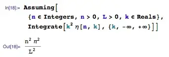
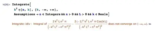
(* Calculate (Δk)^2 = <k^2> - <k>^2 = <k^2> *)
Integrate[
    k^2 η[n, k], {k, -∞, +∞},
    (* Edited: Was: {n ∈ Integers, n > 0}, but this edit didn't
       fix the problem. *) 
    Assumptions -> n ∈ Integers && n > 0]

The problem is that Mathematica can't calculate the last integral for any arbitrary $n$, although it can, correctly, calculate its value for hardcoded $n$s. Like $n=1,2,...$.

My question is: Do you have any idea on how I could calculate it, perhaps by rewriting it a bit, or by using some other trick? In case it helps, the result should be $n^2\pi^2$.

Note: Actually it can be calculated with Cauchy's residue theorem, but I'd like to avoid taking that route, if possible. Though, if it can't be done otherwise, I will post a solution with residual calculation so that this question has an answer.

Mathematica.SE related (to the physical problem) questions:

Is there a more mathematica-y way to label these plots?

Why does FourierTransform converge while same integral manually written does not?

Answer 1

This is a stupid workaround. Anyway:

FindSequenceFunction@Table[Integrate[k^2 η[n, k], {k, -∞, +∞}, Assumptions -> {n == p}], {p, 5}]
(*
 π^2 #1^2 &
*)

Answer 2

The following code yields the correct result:

Another interesting fact is that if I omit the assumption that k ∈ Reals, then Mathematica still gets it right, but it takes ~3x more time:

What is puzzling though is that if I use Assumptions with Integrate I don't get the expected result:

I was under the impression that Assuming[{a1,a2,...}, Integrate[...]] was equivalent to Integrate[..., Assumptions -> a1 && a2 && ...].

Could anyone please try to reproduce my results, ideally in a different OS/Mathematica version combination ? That is something other than Mathematica 9.0.1/Mac OSX 10.9 ?

Answer 3

Here's as close as I can get via Mathematica. First, I just simplify the integrand once for all. Having Simplify in the definition of a function could be really slow. Edit: I added the unsimplified versions of the OP's functions, including a substitution of Boole for If, which I omitted to include in the original answer.

u[n_, x_] := Boole[0 <= x <= L] Sqrt[2/L] Sin[n π x/L];
φ[n_, k_] := FourierTransform[u[n, x], x, k, FourierParameters -> {0, -1}];
η[n_, k_] := φ[n, k]\[Conjugate] φ[n, k];

integrand =
  FullSimplify[k^2 \[Eta][n, k],
               {n \[Element] Integers, n > 0, k \[Element] Reals,L > 0}]
(* -((2 k^2 L n^2 \[Pi] (-1 + (-1)^n Cos[k L]))/(k^2 L^2 - n^2 \[Pi]^2)^2) *)

Then, Integrate gets real close, if you make a substitution k -> n k. Since the differential of n k is n dk, you have to multiply the Integrate below by n.

int = n Integrate[integrand /. k -> n k, {k, -Infinity, Infinity}];
Simplify[int, {n \[Element] Integers, n > 0}]

(* ConditionalExpression[
    (L n^2 Pi^2)/Abs[L]^3, 
    L \[Element] Reals && 3 Arg[-L^2] <= 2 \[Pi] && (Re[1/L^2] <= 0 || 1/L^2 \[NotElement] Reals)] *)

Reduce[Last[%]]
(* False *)

The only problem is that the condition in the ConditionalExpression is a contradiction.