Original question
I would like to put a coloured grid behind the following plot:
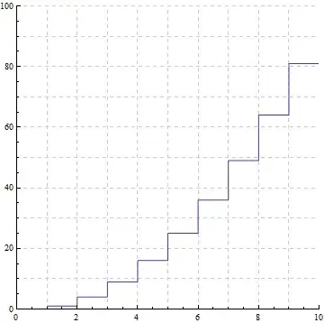
which was generated by:
a = Table[x, {x, 1, 10}];
b = Table[10 x, {x, 1, 10}];
ListLinePlot[{Table[x^2, {x, 1, 10}]}, InterpolationOrder -> 0,
PlotRange -> {{0, 10}, {0, 100}}, GridLines -> {a, b}, GridLinesStyle ->
Directive[GrayLevel[0.8], Dashed], AspectRatio -> 1]
so that I could shade certain squares of the grid so it looks something like:

for example.
Update1
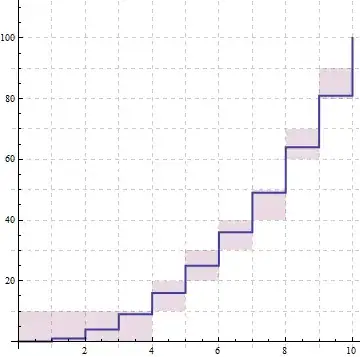
Using Kuba's code below, it is fairly straightforward to overlay an x^2 shaded plot with an x^3 ListLinePlot using the following code:
data = Table[{x, x^2}, {x, 0, 10}];
ceiling = {#, Ceiling[#2 + 1, 10]} & @@@ data;
floor = {#, Floor[#2, 10]} & @@@ data;
a = Table[x, {x, 1, 10}];
b = Table[10 x, {x, 1, 10}];
c = ListLinePlot[{Table[x^3, {x, 1, 10}]}, InterpolationOrder -> 0,
PlotRange -> {{0, 10}, {0, 100}}, GridLines -> {a, b},
GridLinesStyle -> Directive[GrayLevel[0.8], Dashed],
AspectRatio -> 1, PlotStyle -> {Thick}];
Show[ListPlot[{data, ceiling, floor}, InterpolationOrder -> 0,
Joined -> True, AspectRatio -> 1, Filling -> (2 -> {3}),
GridLines -> {Range[10], Range[0, 100, 10]},
GridLinesStyle -> Directive[GrayLevel[0.8], Dashed],
PlotStyle -> {None, None, None}], c]
which generates:

without too much fiddling. Is there a similarly straightforward way of showing a shaded x^3 plot & ListLinePlot x^2 without running into problems with the dimensions of the grid (without fiddling around with the dimensions each time)?
Update2
Thanks to Kuba's code:

with:
lineData[f_, max_, min_: 0] := Table[{x, f[x]}, {x, min, max}];
shadeData[f_, max_, min_: 0] :=
Transpose[{{#, Ceiling[#2 + 1, 10]}, {#, Floor[#2, 10]}} & @@@
Table[{x, f[x]}, {x, min, max}]]

With[{stdOpt = {InterpolationOrder -> 0,
GridLines -> {Range[10], Range[0, 300, 10]},
GridLinesStyle -> Directive[GrayLevel[0.8], Dashed],
Joined -> True, AspectRatio -> 1}},
ListPlot[{lineData[#^2 &, 10], ##} & @@ shadeData[#^3 &, 10],
Filling -> (2 -> {3}), PlotStyle -> {Thick, None, None}, stdOpt,
PlotRange -> {{0, 10}, {0, 100}},

Epilog -> {Red, Opacity[0.5], Rectangle[{1, 10}, {2, 20}], Blue,
Opacity[0.5], Rectangle[{2, 40}, {3, 50}]}

]]
Update3
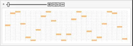
Having some fun with it:
with:
shadeData[f_, max_, min_: 0] :=
Transpose@Table[{{x, Ceiling[f[x] + If[FractionalPart[f[x]] == 0.5, 0.5, 0], 1]},
{x, Floor[f[x], 1]}}, {x, min, max}]

Animate[Quiet[With[{stdOpt = {InterpolationOrder -> 0, GridLines -> {Range[-10, 28,
1], Range[-10, 14]}, GridLinesStyle -> Directive[GrayLevel[0.8], Dashed],
Joined -> True, AspectRatio -> 0.25}}, ListPlot[shadeData[(Sin[# + n])*10 &, 28],
Filling -> (2 -> {1}), FillingStyle -> Directive[Opacity[0.5], Orange],
PlotStyle -> {None, None, None}, stdOpt, Axes -> False, Frame -> False,
ImageSize -> 600, PlotRange -> {{0, 24}, {-10, 10}}]]], {n, 0, 2 \[Pi]},
AnimationDirection -> Forward, AnimationRate -> 0.5]
and

...etc :)

GraphicsandRectanlgeto build this directly, instead of using an existing plotting function. Have you tried this route already? Take a look here. – Szabolcs Nov 20 '13 at 19:02Inset, but it proved to be difficult to position them :/ – martin Nov 20 '13 at 19:04InsetbecauseRectangleis a graphics primitive.Insetis for putting things that are not graphics primitives intoGraphics. Just use aTableto generate the list ofRectangles with appropriate coordinates. – Szabolcs Nov 20 '13 at 19:07Show, &ArrayPlot[Table[GCD[i, j], {i, 10}, {j, 10}]]... no good! - Will go back to your original suggestion - thanks for the other link. – martin Nov 20 '13 at 19:13