Efficiently generating n-D Gaussian random fields

Question

I am interested in an efficient code to generate an $n$-D Gaussian random field (sometimes called processes in other fields of research), which has applications in cosmology.

Attempt

I wrote the following code:

fftIndgen[n_] := Flatten[{Range[0., n/2.], -Reverse[Range[1., n/2. - 1]]}]

Clear[GaussianRandomField];
GaussianRandomField::usage = "GaussianRandomField[size,dim,Pk] returns
a Gaussian random field of size size (default 256)  and dimensions dim 
(default 2) with a powerspectrum Pk";

GaussianRandomField[size_: 256, dim_: 2, Pk_: Function[k, k^-3]] := 
Module[{noise, amplitude, Pk1, Pk2, Pk3, Pk4},
Which[
dim == 1,Pk1[kx_] := 
If[kx == 0 , 0, Sqrt[Abs[Pk[kx]]]]; (*define sqrt powerspectra*)
noise = Fourier[RandomVariate[NormalDistribution[], {size}]]; (*generate white noise*)
amplitude = Map[Pk1, fftIndgen[size], 1]; (*amplitude for all frequels*)
InverseFourier[noise*amplitude], (*convolve and inverse fft*)
dim == 2,
Pk2[kx_, ky_] := If[kx == 0 && ky == 0, 0, Sqrt[Pk[Sqrt[kx^2 + ky^2]]]];
noise = Fourier[RandomVariate[NormalDistribution[], {size, size}]];
amplitude = Map[Pk2 @@ # &, Outer[List, fftIndgen[size], fftIndgen[size]], {2}];
InverseFourier[noise*amplitude],
dim > 2, "Not supported"]
]

Here are a couple of examples on how to use it in one and 2D

GaussianRandomField[1024, 1, #^(-1) &] // ListLinePlot
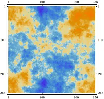
GaussianRandomField[] // GaussianFilter[#, 20] & // MatrixPlot

Question

The performance is not optimal — On other interpreted softwares, such Gaussian random fields can be generated ~20 times faster. Do you have ideas on how to speed things up/improve this code?

Answer 1

Here's a reorganization of GaussianRandomField[] that works for any valid dimension, without the use of casework:

GaussianRandomField[size : (_Integer?Positive) : 256, dim : (_Integer?Positive) : 2,
                    Pk_: Function[k, k^-3]] := Module[{Pkn, fftIndgen, noise, amplitude, s2},
  Pkn = Compile[{{vec, _Real, 1}}, With[{nrm = Norm[vec]},
                                        If[nrm == 0, 0, Sqrt[Pk[nrm]]]], 
                CompilationOptions -> {"InlineExternalDefinitions" -> True}];
  s2 = Quotient[size, 2];
  fftIndgen = ArrayPad[Range[0, s2], {0, s2 - 1}, "ReflectedNegation"];
  noise = Fourier[RandomVariate[NormalDistribution[], ConstantArray[size, dim]]]; 
  amplitude = Outer[Pkn[{##}] &, Sequence @@ ConstantArray[N @ fftIndgen, dim]];
  InverseFourier[noise * amplitude]]

Test it out:

BlockRandom[SeedRandom[42, Method -> "Legacy"]; (* for reproducibility *)
            MatrixPlot[GaussianRandomField[]]
        ]

BlockRandom[SeedRandom[42, Method -> "Legacy"];
            ListContourPlot3D[GaussianRandomField[16, 3] // Chop, Mesh -> False]
            ]

Here's an example the routines in the other answers can't do:

AbsoluteTiming[GaussianRandomField[16, 5];] (* five dimensions! *)
   {28.000959, Null}

Answer 2

If the power spectrum is always of the form $1/k^p$ there are some optimisations you can make. The first is to compile a function to generate the reciprocal of the spectrum: $k^p$. This can be very fast since you don't need to check for the $k=0$ point (the reciprocal spectrum is well behaved at $k=0\ $).

We can then use ReplacePart to temporarily set the value at $k=0$ to something other than 0 (I've used 1), then take the reciprocal to get the spectrum we really wanted, and finally use ReplacePart again to set the value at $k=0$ back to 0.

The other optimisation is to create the random noise directly in frequency space, by having independent normally distributed real and imaginary components. Doing this allows you to get 2 fields at once, from the real and imaginary parts of the complex field which is generated.

The code below is only for 2D, but I think it should generalise to 1D or 3D quite straighforwardly.

The timing to generate 2 fields at 1024 x 1024 is about 280 ms on my PC.

fastpower=Compile[{{n,_Integer},{p,_Real}},
Block[{temp},
temp=Range[-n,n-2,2]^2;
Outer[Plus,temp,temp]^(p/2)]];

spectrum[n_,gamma_]:=ReplacePart[1/ReplacePart[
RotateRight[fastpower[n,-0.5gamma],{n/2,n/2}],
{1,1}->1.],{1,1}->0.];

complexrandoms[n_]:=RandomReal[NormalDistribution[0,1],{n,n}] 
+ I RandomReal[NormalDistribution[0,1],{n,n}]

fields[n_,gamma_]:={Re[#],Im[#]}&@Fourier[complexrandoms[n]spectrum[n,gamma]];

Example:

{f1,f2}=fields[1024,-3];

GraphicsRow[Image@Rescale@#&/@{f1,f2}]

Answer 3

Here is a version of the code which incorporates the compilation suggestion of acl.

fftIndgen[n_] :=  Flatten[{Range[0., n/2.], -Reverse[Range[1., n/2. - 1]]}]

Clear[GaussianRandomField];
GaussianRandomField::usage = " GaussianRandomField[size,dim,Pk] 
returns a Gaussian random field of size size (default 256)
and dimensions dim (default 2) with a powerspectrum Pk default k^(-3))";
GaussianRandomField[size_: 256, dim_: 2, Pk_: Function[k, k^-3]] := 
Module[{noise, amplitude, Pk1, Pk2, Pk3,Pk4,kx,ky,kz,ku},
Which[
dim == 1,
Pk1 = Compile[{{kx, _Real}}, 
 If[kx == 0 , 0, Sqrt[Abs[Pk[kx]]]]]; (*define sqrt powerspectra*)
 noise = Fourier[RandomVariate[NormalDistribution[], {size}]]; (*generate white noise*)
 amplitude = Map[Pk1, fftIndgen[size], 1]; (*amplitude for all frequels*)
InverseFourier[noise*amplitude]//Chop, (*convolve and inverse fft*)
dim == 2,
Pk2 = Compile[{{kx, _Real}, {ky, _Real}},If[kx == 0 && ky == 0, 0,
  Sqrt[Pk[Sqrt[kx^2 + ky^2]]]]];
noise = Fourier[RandomVariate[NormalDistribution[], {size, size}]];
amplitude = Map[Pk2 @@ # &, Outer[List, fftIndgen[size], fftIndgen[size]], {2}];
InverseFourier[noise*amplitude]//Chop,
dim == 3,
Pk3 = Compile[{{kx, _Real}, {ky, _Real}, {kz, _Real}},
 If[kx == 0 && ky == 0 && kz == 0, 0, Sqrt[Pk[Sqrt[kx^2 + ky^2 + kz^2]]]]];
noise = 
Fourier[RandomVariate[NormalDistribution[], {size, size, size}]];
amplitude = Map[Pk3 @@ # &, 
 Outer[List,fftIndgen[size],fftIndgen[size],fftIndgen[size]], {3}];
InverseFourier[noise*amplitude]//Chop,
dim == 4,
Pk4 = Compile[{{kx, _Real}, {ky, _Real}, {kz, _Real}, {ku,_Real}},If[
kx == 0 && ky == 0 && kz == 0 && ku == 0, 0,  Sqrt[Pk[Sqrt[kx^2 + ky^2 + kz^2 + ku^2]]]]];
noise = 
Fourier[RandomVariate[NormalDistribution[], {size, size, size, size}]];
amplitude = 
Map[Pk4 @@ # &, 
 Outer[List, fftIndgen[size], fftIndgen[size], fftIndgen[size], 
  fftIndgen[size]], {4}];
InverseFourier[noise*amplitude]//Chop,
dim > 4, "Not supported"]
]

We can check that the GRF has the correct powerspectrum via the command

lm = {Range[128], 
  Map[Mean, 
    Table[Fourier[GaussianRandomField[256, 1, #^(-3/2) &]] // 
        Abs // #^2 &, {5}] // Transpose] // 
   Take[#, {2, 256/2 + 1}] &} // Transpose // Log // 
LinearModelFit[#, {1, x}, x] &;
lm["ParameterTable"]

An example

GaussianRandomField[] // MatrixPlot

It can also be used to generate cloud-like images

u = GaussianRandomField[] // GaussianFilter[#, 1] &;Image[u] // ImageAdjust

Finally a 3D Example

GaussianRandomField[16, 3] // Chop // ListContourPlot3D

In terms of performance we have

GaussianRandomField[128, 3]; // AbsoluteTiming
{7.169987,Null}

Answer 4

While I did not have time to do any major reorgnization, let me demonstrate one cheap way to speed this up, namely, compilation. I'll do it for the 1d case for simplicity.

fftIndgen[n_] := Flatten[{Range[0., n/2.], -Reverse[Range[1., n/2. - 1]]}]

grf1[size_,pk_] :=
    Module[ {noise,amplitude,Pk1},
    (*Pk1[kx_] :=If[ kx == 0,0,Sqrt[Abs[pk[kx]]]]; (*define sqrt powerspectra*)*)
        With[ {pkt = pk},
            Pk1 = Compile[{{kx,_Real}},
                If[ kx == 0,
                    0,
                    Sqrt[Abs[pkt[kx]]]
                ]
            ]
        ];
        noise = Fourier[RandomVariate[NormalDistribution[], {size}]]; (*generate white noise*)
        amplitude = Map[Pk1, fftIndgen[size], 1]; (*amplitude for all frequels*)
        InverseFourier[noise*amplitude]
    ]

Assuming I did not break anything, this is 5-6 times faster:

GaussianRandomField[2^19, 1, #^(-1) &]; // AbsoluteTiming
grf1[2^19, #^(-1) &]; // AbsoluteTiming
(*{1.755694, Null}
{0.281733, Null}*)

All I did here is compile the Pk1 function (the use of With is to inject the argument into the body to be compiled; maybe it's not necessary, but I did not check).

Answer 5

I know, it's long a ago. I just stumbled into this post and cannot resist. JM's code can be sped up even more, even without Compile: First, we can employ Outer in conjunction with Plus to compute the squared norms of frequencies at once. Second, only the zero frequency makes problems when applying Pk, so we can set its squared norm temporarily to 1. and use vectorization when we apply Pk. (Edit: I just realize that Simon Woods had the same idea...) That leads to a roughly 18-fold speed up on my machine for the whole routine (with size = 1024). (Another curiosity is that applying Sqrt twice is faster than applying Power[#,1/4]& once - probably due to hardware optimization.)

GaussianRandomField2[
  size : (_Integer?Positive) : 256, dim : (_Integer?Positive) : 2, 
  Pk_: Function[k, k^-3]] := Module[{Pkn, fftIndgen, noise, amplitude, s2},
  s2 = Quotient[size, 2];
  fftIndgen = N@ArrayPad[Range[0, s2], {0, s2 - 1}, "ReflectedNegation"];
  amplitude = Sqrt[Outer[Plus, Sequence @@ ConstantArray[fftIndgen^2, dim], dim]];
  amplitude[[Sequence @@ ConstantArray[1, dim]]] = 1.;
  amplitude = Pk[amplitude];
  amplitude[[Sequence @@ ConstantArray[1, dim]]] = 0.;
  noise = Fourier[RandomVariate[NormalDistribution[], ConstantArray[size, dim]]];
  Re[InverseFourier[noise amplitude]]
  ]
SeedRandom[666];
a = GaussianRandomField[1024]; // AbsoluteTiming
SeedRandom[666];
b = GaussianRandomField2[1024]; // AbsoluteTiming
Max[Abs[a - b]]

{1.29018, Null}

{0.069911, Null}

2.72278*10^-18