Solve trigonometric equation

Question

I'm looking for a solution (graphic, numeric or analytic) for a function of the form:

$$a^2\tanh(x)=\tan(ax),\quad a ≥ 1,\ x > 0$$

preferably using Mathematica. Any advice?

Answer 1

We will show:

• How to reproduce and improve the WolframAlpha plot, and what it shows about the problem
• How to use NDSolve to approximate the function
• How to use FindRoot to improve an NDSolve solution (necessary for the first root)
• How to define x as a function of a, for a >= 0

Here is a plot some of the solutions. (We omit the trivial solution x[a_] := 0, as in the OP.)

WolframAlpha

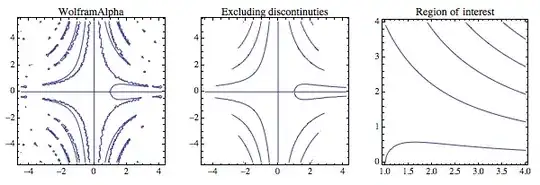
WolframAlpha makes a very rough picture, which is roughly equivalent to the first contour plot. We can improve upon this by excluding the discontinuities where Cos[a * x] == 0 or a * x == (2 k + 1) π/2; further, we can find the missing branches in the region of interest (a >= 1, x > 0) by increasing the number of PlotPoints.

Block[{a1, a2, x1, x2},
 {a1, a2} = {-4.492122341961456`, 4.186102420126525`};
 {x1, x2} = {-5.314327054433177`, 5.314327054433177`};
 GraphicsRow[
  {ContourPlot[a^2*Tanh[x] - Tan[a*x] == 0, {a, a1, a2}, {x, x1, x2},
    PlotLabel -> "WolframAlpha"],
   ContourPlot[a^2*Tanh[x] - Tan[a*x] == 0, {a, a1, a2}, {x, x1, x2},
    Exclusions -> Cos[a*x] == 0, 
    PlotLabel -> "Excluding discontinuties"],
   ContourPlot[{a^2*Tanh[x] == Tan[a*x]}, {a, 1, 4}, {x, 0, 4},
    PlotPoints -> 50, Exclusions -> Cos[a*x] == 0, 
    PlotLabel -> "Region of interest"]},
  ImageSize -> 600]
 ]

However, there will be limit to how far one can increase the quality of the plot, and not just because of the time it takes. The reason is that the regions in which the function is negative grow vanishingly thin as a increases, making it unlikely for ContourPlot to find points where the function changes sign. This can be seen in both plots below. Indeed, the plot on the right shows that an inflection in the graph develops, which can confuse FindRoot, if it is not supplied with good initial points. This makes using Table and FindRoot to create an Interpolation difficult. It will be easier to use NDSolve. (Note that the sought-after solutions are where green switches to red; the white parts are the excluded discontinuities.)

Row[{
  ContourPlot[a^2*Tanh[x] - Tan[a*x], {a, 0, 4}, {x, 0, 4}, 
   Contours -> {0}, Exclusions -> Cos[a*x] == 0, 
   ColorFunction -> "RedGreenSplit", 
   ContourStyle -> {Thickness[Medium], Blue}, ImageSize -> 225], " ",
  Plot3D[a^2*Tanh[x] - Tan[a*x], {a, 0, 4}, {x, 0, 4}, 
   PlotPoints -> 100, Exclusions -> Cos[a*x] == 0, 
   MeshFunctions -> {Function[{a, x, f}, f]}, Mesh -> {{0}}, 
   MeshStyle -> {Thick, Blue}, MeshShading -> (ColorData["RedGreenSplit"] /@ {0, 1}), 
   PlotRange -> {-10, 20}, ImageSize -> 350, ViewPoint -> {10, -1, 1}]
  }]

Solving for the curve using NDSolve

There are two things I long for (which means I do not think they are available as built-in features): 1) A function that returns an interpolation of a branch of the solution to an equation, and 2) a way to pass NDSolve an extra error measure to be minimized.

One can set up a differential equation for an integral curve on a surface from the gradient of its equation. In this case, we are seeking a level set, so our differential equation results from differentiating the equation, treating x and as function a (or vice versa as desired):

D[a^2 * Tanh[x[a]] - Tan[a * x[a]], a] == 0

To get a level curve we feed NDSolve an initial point on it, which we can find with FindRoot. There is a solution x[a] below each discontinuity Cos[a * x] == 0. Thus at a == 1, the discontinuity is at x == (2 k + 1) π/2. For the sake of an example, we'll choose x == 3 π/2 and initial value x0 just below it.

FindRoot[a^2*Tanh[x0] - Tan[a*x0] /. a -> 1, {x0, 3 π/2 - 0.1}]
  (* {x0 -> 3.9266} *)

NDSolveValue[
  {D[a^2*Tanh[x[a]] - Tan[a*x[a]], a] == 0, 
   x[1] == (x0 /. FindRoot[a^2*Tanh[x0] - Tan[a*x0] /. a -> 1, {x0, 3 π/2 - 0.1}])}, 
  x, {a, 1, 10}];
Plot[%[a], {a, 1, 10}, Axes -> False, Frame -> True]

Using FindRoot to correct the first solution

The above approach works for the other branches except the one below a * x == π/2. The differential equation is indeterminate at a = 1, x = 0, so we will start by fudging a little and then correct the errors. For the initial value for x[1], we find a root for a nearby a with x < π/2/a. Note the value of this solution at a = 1 is far from the correct value 0.

FindRoot[a^2*Tanh[x0] - Tan[a*x0] /. a -> 1.1, {x0, π/2/1.1 - 0.1}]
  (* {x0 -> 0.358323} *)

sol0 = NDSolveValue[
   {D[a^2*Tanh[x[a]] - Tan[a*x[a]], a] == 0, 
    x[1] == (x0 /. FindRoot[a^2*Tanh[x0] - Tan[a*x0] /. a -> 1.1, {x0, π/2/1.1 - 0.1}])},
   x, {a, 1, 10}];
sol0[1]
Plot[sol0[a], {a, 1, 10}, Axes -> False, Frame -> True]

  (* 0.358323 *)

This can be corrected with FindRoot. The output of NDSolve is an InterpolatingFunction (say, ifn) that has for a certain grid of domain values (accessed via ifn["Grid"]), corresponding values of the solution (accessed via ifn["ValuesOnGrid"]). We can improve the solution by improving the values on the grid.

sol0Imp = Interpolation @ Transpose @ 
     {sol0["Grid"], 
      MapThread[
       x0 /. FindRoot[a^2*Tanh[x0] - Tan[a*x0] /. a -> #1, {x0, #2}] &,
       {First /@ sol0["Grid"], sol0["ValuesOnGrid"]}]};
sol0Imp[1]
Plot[sol0Imp[a], {a, 1, 10}, Axes -> False, Frame -> True]
  (* 1.2661*10^-8 *)

The other branches normally do not need this improvement. NDSolve does a good job approximating them.

Defining the functions

We will label the branches k = 0, 1, 2, ..., where k corresponds to the branch below a * x == (2k + 1) π/2. Here I randomly chose the domain 1 <= a <= 10. One can change it, or as shown below, have the domain automatically extended. The result of NDSolve is memoized, so that it is a one-time cost for each k.

xfn[0] := xfn[0] = Module[{sol, a, a0 = 1.1, x, x0},
    sol = NDSolveValue[
       {D[a^2*Tanh[x[a]] - Tan[a*x[a]], a] == 0, 
        x[1] == (x0 /. FindRoot[a^2 * Tanh[x0] - Tan[a * x0] /. a -> a0,
                                {x0, π/2/a0 - 0.1}])},
       x, {a, 1, 10}];
    Interpolation @ Transpose @
      {sol["Grid"], 
       MapThread[
        x0 /. FindRoot[a^2 * Tanh[x0] - Tan[a * x0] /. a -> #1, {x0, #2}] &,
        {First /@ sol["Grid"], sol["ValuesOnGrid"]}]}
    ];
xfn[k_] := xfn[k] = Block[{a, x, x0},
   NDSolveValue[
     {D[a^2 * Tanh[x[a]] - Tan[a*x[a]], a] == 0, 
      x[1] == (x0 /. FindRoot[a^2 * Tanh[x0] - Tan[a * x0] /. a -> 1,
                              {x0, (2k + 1) π/2 - 0.1}])},
     x, {a, 1, 10}]
   ]

The output of the plot is shown above. One can see that this procedure is reasonably fast. The second plot if faster because of memoization, and the difference shows the time it takes to compute the 20 solutions.

Plot[Evaluate@Table[xfn[k][a], {k, 0, 19}], {a, 1, 8},
   Axes -> False, Frame -> True, PlotRange -> {0, 8}, PlotRangePadding -> Scaled[0.02], 
   AspectRatio -> 1]; // Timing
  (* {0.339130, Null} *)

Plot[Evaluate@Table[xfn[k][a], {k, 0, 19}], {a, 1, 8},
   Axes -> False, Frame -> True, PlotRange -> {0, 8}, PlotRangePadding -> Scaled[0.02], 
   AspectRatio -> 1]; // Timing
 (* {0.048151, Null} *)

Automatically extending the domain

Here is a way to extend the domain. We use NDSolve to fill in the next segment of the domain, restarting it from where it left off, and stitch the old and new interpolations together. The next segment extends from the old endpoint to 10. times that endpoint (1., 10., 100., etc.). The new interpolation replaces the old one in xfn0[k]. There is a small overhead in checking that the argument a to xfn[k] is in the currently defined domain (conveniently stored in the InterpoltingFunction xfn0[k]), which does not noticeably affect the timing of the plot above.

ClearAll[xfn, xfn0]; (* redefine xfn *)
xfn0[k_]["Domain"] := {{1., 1.}};
xfn0[k_]["Grid"] := {};
xfn0[k_]["ValuesOnGrid"] := {};
xfn0[0, {1., 10.}] := xfn0[0] = Module[{sol, a, a0 = 1.1, x, x0},
    sol = NDSolveValue[
           {D[a^2*Tanh[x[a]] - Tan[a*x[a]], a] == 0, 
            x[1] == (x0 /. FindRoot[a^2 * Tanh[x0] - Tan[a * x0] /. a -> a0,
                                    {x0, π/2/a0 - 0.1}])},
           x, {a, 1, 10}];
    Interpolation @ Transpose @
      {sol["Grid"], 
       MapThread[
        x0 /. FindRoot[a^2 * Tanh[x0] - Tan[a * x0] /. a -> #1, {x0, #2}] &,
        {First /@ sol["Grid"], sol["ValuesOnGrid"]}]}
    ];
xfn0[k_, {a1_, a2_}] := xfn0[k] = Module[{sol, a, x, x0, x1},
    If[xfn0[k]["Domain"][[1, 2]] == 1.,

      x1 = x0 /. FindRoot[a^2*Tanh[x0] - Tan[a*x0] /. a -> 1., {x0, (2 k + 1) π/2 - 0.1}];
      xfn0[k]["Grid"] = {{1.}};
      xfn0[k]["ValuesOnGrid"] = {x1},

      x1 = Last@xfn0[k]["ValuesOnGrid"]
     ];
    sol = NDSolveValue[{D[a^2*Tanh[x[a]] - Tan[a*x[a]], a] == 0, x[a1] == x1},
                       x, {a, a1, a2}];
    Interpolation @ Transpose @
      {Join[xfn0[k]["Grid"], Rest@sol["Grid"]], 
       Join[xfn0[k]["ValuesOnGrid"], Rest@sol["ValuesOnGrid"]]}
    ];
xfn[k_][a_] /; 1 <= a < xfn0[k]["Domain"][[1, 2]] := xfn0[k][a];
xfn[k_][a_?NumericQ] := (xfn0[k, xfn0[k]["Domain"][[1, -1]] {1., 10.}]; xfn[k][a]);

xfn[0][1]
  (* 1.2661*10^-8 *)

xfn[0][1132]
  (* 0.00138714 *)

Answer 2

Numerically (using FindRoot as you do):

fn[x_, a_] := a^2*Tanh[x] - Tan[a*x]
xmax = 5;
firstSol[a_] := First@Select[N@Sort@DeleteDuplicates@Rationalize[Quiet@Chop@
     FindRoot[fn[x, a] == 0, {x, Range[0.1, xmax, 0.1]}][[1, 2]],10^-10], # >= .1 &]

Then you can either Manipulate or Table:

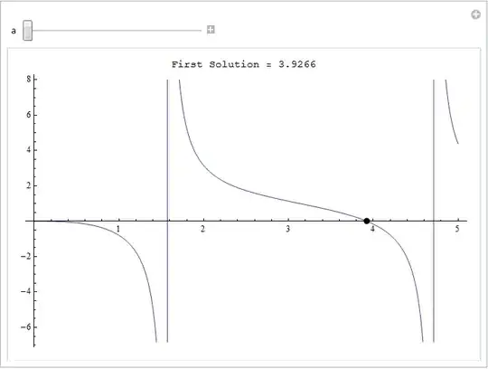
Manipulate[Column[{"First Solution = " <> ToString@firstSol[a],Plot[fn[x, a], {x, 0, 5},
  ImageSize -> 500,Epilog -> {PointSize[Large], Point[{firstSol[a], 0}]}]},
  Alignment -> Center], {a, 1, 5, 1}]

Or:

Table[firstSol@a, {a, 1, 5}]

{3.9266, 0.555377, 0.435336, 0.346333, 0.285585}

Although xmax and the domain in which you want to find solutions has to be chose carefully. In your function a has a big influence.

Answer 3

Here is a solution that give the root in the kth segment :

root[a_,k_] := FixedPoint[(k Pi + ArcTan[a^2 Tanh[#]])/a &, k Pi +1/2]

root[2.73, #] & /@ Range[0, 3]

{0.465728, 1.67378, 2.82772, 3.97879}

Edit

Thanks to Öska's remarks, here is a more robust solution :

root[a_, k_] := 
 FixedPoint[(k Pi + ArcTan[a^2 Tanh[#]])/a &,
             k Pi + 0.5,   
             SameTest -> (Abs[#1 - #2] < 10^-8 &)
           ]

Answer 4

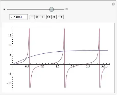
Here's a simple way to eyeball things:

Manipulate[Plot[{a^2 Tanh[x], Tan[a x]}, {x, 0, Pi}], {a, 1, Pi}]