How to solve for the intersection points of two ellipses?

Question

I have a parametric equation of two ellipses as follow

$\begin{cases} x=a_1 \text{sin$\theta $}+b_1 \text{cos$\theta $}+c_1 \\ y=d_1 \text{sin$\theta $}+e_1 \text{cos$\theta $}+f_1 \\ \end{cases}$

$\begin{cases} x=a_2 \text{sin$\theta $}+b_2\text{cos$\theta $}+c_2 \\ y=d_2 \text{sin$\theta $}+e_2 \text{cos$\theta $}+f_2 \\ \end{cases}$

Now I want to solve the intersection point coordinates and visualize them.

My trial

Here, mat1 owns the style {{a1,b1,c1},{d1,e1,f1}}.

solvePoints0[mat1_, mat2_] :=
 Module[{sol, θValue, θ, ptRule},
  sol =
   Solve[
    Thread[
     mat1.{Sin[θ1], Cos[θ1], 1} ==
      mat2.{Sin[θ2], Cos[θ2], 1}], {θ1, θ2}];
  θValue = Mod[(#[[1, 2, 1]] & /@ sol) /. C[1] -> 1., 2 Pi];
  ptRule = List /@ Thread[θ -> θValue];
  Cases[
   mat1.{Sin[θ], Cos[θ], 1} /. ptRule,{_Real, _Real}]
 ]

showEllipse0[mat1_, mat2_, opts : OptionsPattern[]] :=
 With[{pts = solvePoints0[mat1, mat2]},
   ParametricPlot[
    {mat1.{Sin[θ], Cos[θ], 1}, 
     mat2.{Sin[θ], Cos[θ], 1}}, {θ, 0, 2 Pi},
    Epilog -> {PointSize[Large], Red, Point[pts]},
    Evaluate[
     Sequence @@ FilterRules[{opts}, Options[ParametricPlot]]]
   ]
  ] /; MatrixQ[mat1, NumericQ] && MatrixQ[mat2, NumericQ]

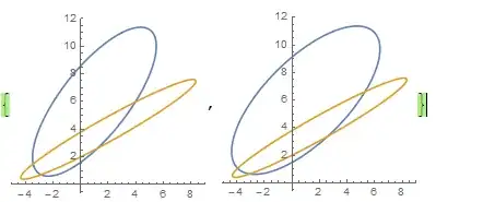
Test

showEllipse0[##, ImageSize -> 200] & @@@
 {{{{1, 2, 1}, {2, 3, 4}}, {{2, 2, 2}, {3, 2, 4}}},
  {{{3, 1, 1}, {2, 3, 4}}, {{4, 2, 2}, {3, 4, 4}}},
  {{{3, 2, 1}, {2, 3, 4}}, {{2, 2, 2}, {3, 2, 4}}},
  {{{2, 1, 1}, {2, 3, 4}}, {{4, 1, 2}, {3, 2, 4}}}}

However, solvePoints0 has a bug

solvePoints0[{{4, 2, 1}, {2, 5, 6}}, {{6, 2, 2}, {3, 2, 4}}]
solvePoints0[{{5, 2, 1}, {2, 5, 6}}, {{6, 2, 2}, {3, 2, 4}}]

{}
{}

In fact, they have intersection point coordinates.

showEllipse0 @@@
 {{{{4, 2, 1}, {2, 5, 6}}, {{6, 2, 2}, {3, 2, 4}}},
  {{{5, 2, 1}, {2, 5, 6}}, {{6, 2, 2}, {3, 2, 4}}}}

To fixed this bug, I rewrite the function solvePoints0 using NSolve

solvePoints[mat1_, mat2_] :=
 Module[
   {sol, θValue, θ, ptRule},
   sol =
    Quiet@
      NSolve[
        Thread[
         mat1.{Sin[θ1], Cos[θ1], 1.} ==
          mat2.{Sin[θ2], Cos[θ2], 1.}], {θ1, θ2}] /. C[1] -> 1.;
   θValue = #[[1, 2]] & /@ sol;
   ptRule = List /@ Thread[θ -> θValue];
   Cases[
    mat1.{Sin[θ], Cos[θ], 1} /. ptRule, {_Real, _Real}]
 ] /; MatrixQ[mat1, NumericQ] && MatrixQ[mat2, NumericQ]

Now,

solvePoints[{{4, 2, 1}, {2, 5, 6}}, {{6, 2, 2}, {3, 2, 4}}]
solvePoints[{{5, 2, 1}, {2, 5, 6}}, {{6, 2, 2}, {3, 2, 4}}]

Question

• I think my methods is fussy and bad, so I would like to know how to solve this question in a elegant way.

---

Update

Thanks for J.M's suggestions, with the help of Graphics`Mesh`FindIntersections

newSolution[mat1_, mat2_] :=
 Module[{graph, pts},
  graph =
   ParametricPlot[
    {mat1.{Sin[θ], Cos[θ], 1},
     mat2.{Sin[θ], Cos[θ], 1}}, {θ, 0, 2 Pi},Epilog -> {Point[{.1, .2}]}];
  pts = Graphics`Mesh`FindIntersections[First[graph]];
  graph /.
   (Epilog -> _) -> Epilog -> {Red, PointSize[Medium], Point[pts]}
]

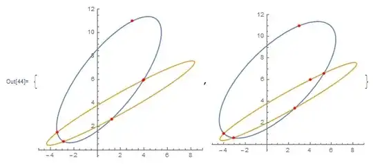
Test

newSolution[##] & @@@ 
 {{{{1, 2, 1}, {2, 3, 4}}, {{2, 2, 2}, {3, 2, 4}}}, 
  {{{3, 1, 1}, {2, 3, 4}}, {{4, 2, 2}, {3, 4, 4}}}, 
  {{{3, 2, 1}, {2, 3, 4}}, {{2, 2, 2}, {3, 2, 4}}}, 
  {{{2, 1, 1}, {2, 3, 4}}, {{4, 1, 2}, {3, 2, 4}}}}

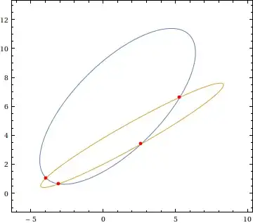
newSolution @@@ 
 {{{{4, 2, 1}, {2, 5, 6}}, {{6, 2, 2}, {3, 2, 4}}},
  {{{5, 2, 1}, {2, 5, 6}}, {{6, 2, 2}, {3, 2, 4}}}}

Obviously, this is not a good method owning to that it cannot find the intersection points correctly.

Answer 1

Alright, I managed to borrow a computer. Here's an implementation of my suggestion:

ellipseIntersections[mat1_?MatrixQ, mat2_?MatrixQ] /; 
       Dimensions[mat1] == Dimensions[mat2] == {2, 3} :=
{\[FormalX], \[FormalY]} /. 
RootReduce[Solve[Flatten[Map[
      GroebnerBasis[Append[Thread[{\[FormalX], \[FormalY]} == #],
                           \[FormalC]^2 + \[FormalS]^2 == 1],
                    {\[FormalX], \[FormalY]}, {\[FormalC], \[FormalS]}] &,
    {mat1, mat2}.{\[FormalC], \[FormalS], 1}]] == 0,
{\[FormalX], \[FormalY]}, Reals]]

where, apart from the use of GroebnerBasis[], I use formal symbols for safety, and add validity checks for the arguments. I use the combination RootReduce[Solve[(* stuff *)]] to generate exact coordinates; replace this with NSolve[] if you only want numerical approximations.

Before demonstrating this function, allow me to show a different way to render your ellipses. Here, I have chosen to use the NURBS (that is, BSplineCurve[]) representation of a circle, along with a suitable affine transformation. Thus:

makeEllipse[mat_?MatrixQ] /; Dimensions[mat] == {2, 3} := Module[{aff},
    aff = AffineTransform[{Drop[mat, None, -1], mat[[All, -1]]}];
    BSplineCurve[aff /@ {{1, 0}, {1, 1}, {-1, 1}, {-1, 0},
                         {-1, -1}, {1, -1}, {1, 0}},
                 SplineClosed -> True, SplineDegree -> 2, 
                 SplineKnots -> {0, 0, 0, 1/4, 1/2, 1/2, 3/4, 1, 1, 1}, 
                 SplineWeights -> {1, 1/2, 1/2, 1, 1/2, 1/2, 1}]]

Now, pictures!

e1 = {{5, 2, 1}, {2, 5, 6}}; e2 = {{6, 2, 2}, {3, 2, 4}};
Graphics[{{RGBColor[7/19, 37/73, 22/31], makeEllipse[e1]},
          {RGBColor[59/67, 11/18, 1/7], makeEllipse[e2]},
          {Red, AbsolutePointSize[5], Point[ellipseIntersections[e1, e2]]}},
         Frame -> True]

Here's the case e1 = {{1, 2, 1}, {2, 3, 4}}; e2 = {{2, 2, 2}, {3, 2, 4}};:

which shows that ellipseIntersections can deal with tangencies.