516

Recently I have learned how to draw simple stuff with TikZ. I really like it. Now I wonder if it is possible to draw with TikZ on a image. Instead of pasting a image in Illustrator and adding some vectors to point something in the picture I would like to do it using TikZ. Is it possible?

For example, on a picture of a computer (PNG,etc) I would like to draw some arrows and labels saying "Keyboard", "Monitor", etc.

g.kov
  • 21,864
  • 1
  • 58
  • 95
nacho4d
  • 11,093
  • 5
    a couple of years later: Ignasi asked me to add a link to the related answer http://tex.stackexchange.com/questions/38632/image-with-axis/38634#comment355583_38634 – Christian Feuersänger Jan 25 '14 at 20:04

8 Answers8

558

(The first part of this answer is taken from my answer to a similar—but not identical—question.)

You can put an \includegraphics inside a TikZ node and then draw over it. The following code adds the picture so that the lower left corner is at the origin of the TikZ coordinate system.

\documentclass[tikz]{standalone}
\begin{document}
\begin{tikzpicture}
    \node[anchor=south west,inner sep=0] at (0,0) {\includegraphics[width=\textwidth]{some_image.jpg}};
    \draw[red,ultra thick,rounded corners] (7.5,5.3) rectangle (9.4,6.2);
\end{tikzpicture}
\end{document}

With a picture from Wikipedia as some_image.jpg, this yields

example

There is a slight problem with this solution: whenever you choose to scale the image differently (e.g. with width=0.9\textwidth), you have to correct the coordinates for your annotations. So it might be useful to introduce coordinates relative to the picture:

\documentclass[tikz]{standalone}
\begin{document}
\begin{tikzpicture}
    \node[anchor=south west,inner sep=0] (image) at (0,0) {\includegraphics[width=0.9\textwidth]{some_image.jpg}};
    \begin{scope}[x={(image.south east)},y={(image.north west)}]
        \draw[red,ultra thick,rounded corners] (0.62,0.65) rectangle (0.78,0.75);
    \end{scope}
\end{tikzpicture}
\end{document}

Then inside the scope, (0,0) is at the lower left of the picture and (1,1) is at the upper right and scaling the picture automatically scales the annotations (or more correctly, it scales their places; the line width and text size stays the same).

A small warning: If you want to draw circles in the new coordinate system, you have to use a radius with absolute lengths (e.g. [radius=1cm]). Otherwise the circle will become an ellipse (if the image is not square).

Display Name
  • 46,933
Caramdir
  • 89,023
  • 26
  • 255
  • 291
  • 14
    I didn't now that x={(image.south east)},y={(image.north west)} is possible! Thanks, I used
     `\pgfsetxvec{\pgfpointanchor{image}{south east}}%`
     `\pgfsetyvec{\pgfpointanchor{image}{north west}}%`


    so far in my implementation.

    – Martin Scharrer Jan 24 '11 at 08:56
  • Is there a way to make the scope square? So that only the width goes from 0 to 1? – Geoff Apr 19 '11 at 20:36
  • 5
    @Geoff: I finally got around to implement an option for this. The code is available at the tex-sx bzr repository. To use it, download the onimage.dtx file and run pdflatex on it to obtain the onimage.sty and the documentation. (Eventually the package will be available over CTAN.) – Caramdir Jul 04 '11 at 12:01
  • I'm finally trying to compile this, and I get "Undefined control sequence." on lines with \tse (l.115). Thanks for any help. – Geoff Nov 10 '11 at 20:42
  • @Geoff: You mean the code from launchpad? What did you do exactly? – Caramdir Nov 11 '11 at 01:28
  • 1
    You could also define two additional commands as stated her: http://kogs-www.informatik.uni-hamburg.de/~meine/tikz/, then the coordinates of the drawing over the image can be set in image coordinates, something I used extensively in my PhD-thesis... – Habi Jul 10 '12 at 14:04
  • Thanks for the answer! Say, instead of using rectangle as noted, one wants to use to use something like \node[minimum width=0.2\imagewidth]; what would be the best way to extract the width \imagewidth of node (image) in this kind of approach? – sdaau Mar 31 '14 at 17:00
  • I just generalized the approach presented here, because this one here relies on the south west anchor being in(0,0)` for the image; see my extended version (unsing relative coordinates in two images/nodes) http://tex.stackexchange.com/a/214390/8042 – Ronny Nov 28 '14 at 08:39
  • 10
    4 years later, onimage is still not on CTAN. Would you please consider uploading it? It is such a useful package! – AlexG Feb 24 '15 at 11:32
  • how do i write text on the image ? – Kong Jan 12 '21 at 18:00
  • @Kong Using TikZ nodes. – AlexG Jul 29 '21 at 13:49
508

This is meant to be an addition to Caramdir's answer, but I cannot figure out how to insert line breaks into comments:

To make it easier to find the desired points in the new coordinate system, you can draw a labeled grid on top of the image while you're working on it:

\draw[help lines,xstep=.1,ystep=.1] (0,0) grid (1,1);
\foreach \x in {0,1,...,9} { \node [anchor=north] at (\x/10,0) {0.\x}; }
\foreach \y in {0,1,...,9} { \node [anchor=east] at (0,\y/10) {0.\y}; }

image with grid

Complete example:

\documentclass[tikz]{standalone}
\begin{document}
\begin{tikzpicture}
    \node[anchor=south west,inner sep=0] (image) at (0,0) {\includegraphics[width=0.9\textwidth]{some_image.jpg}};
    \begin{scope}[x={(image.south east)},y={(image.north west)}]
        \draw[help lines,xstep=.1,ystep=.1] (0,0) grid (1,1);
        \foreach \x in {0,1,...,9} { \node [anchor=north] at (\x/10,0) {0.\x}; }
        \foreach \y in {0,1,...,9} { \node [anchor=east] at (0,\y/10) {0.\y}; }
    \end{scope}
\end{tikzpicture}
\end{document}
anderstood
  • 2,196
  • 19
  • 35
Jake
  • 232,450
120

For PSTricks fans, the solution is also simple. Unlike Caramdir's and Jake's solutions which use decimal numbers for normalization, I use integer instead. I believe that using integer is better. :-)

There are three steps as follows:

  1. Specify the number of columns and rows. Higher values ease you to determine positions more accurately. Unless you are happy to redo the third step, avoid changing these values after completing the third step.
  2. Specify the scale. Scaling does not affect what you have done in the third step.
  3. Superimposing is done here. To enable the grid, change showgrid from false to top. The grid will be useful to determine positions.
\documentclass[pstricks,border=12pt]{standalone}

\def\M{4}% columns
\def\N{4}% rows
\def\scale{0.25}% scale
\def\filename{mycena_interrupta}% filename


\usepackage{graphicx}
\newsavebox\IBox
\savebox\IBox{\includegraphics[scale=\scale]{\filename}}

\addtopsstyle{gridstyle}
{
    gridcolor=yellow,
    subgridcolor=gray,
    subgriddiv=10,
    griddots=0,
    subgriddots=5,
    gridwidth=0.4pt,
    subgridwidth=0.2pt,
}

\psset
{
   xunit=0.5\dimexpr\wd\IBox/\M,
   yunit=0.5\dimexpr\ht\IBox/\N,
}

\begin{document}
\begin{pspicture}[showgrid=top](-\M,-\N)(\M,\N)
    \rput(0,0){\usebox\IBox}
    \psframe[linecolor=red,linewidth=2pt,dimen=inner,framearc=0.5](0.9,1.2)(2.2,2)
\end{pspicture}
\end{document}

When showgrid=top:

enter image description here

The final result with showgrid=false:

enter image description here

60

enter image description here

MWE using Asymptote graphic() label:

% igrid.tex
\documentclass{article}
\usepackage[inline]{asymptote}
\usepackage{lmodern}
\begin{document}
\begin{figure}
\begin{asy}
import graph;
import math;

defaultpen(fontsize(10pt));
real sc=2;
unitsize(sc*1bp);
real wd=200*sc;
real ht=120*sc;

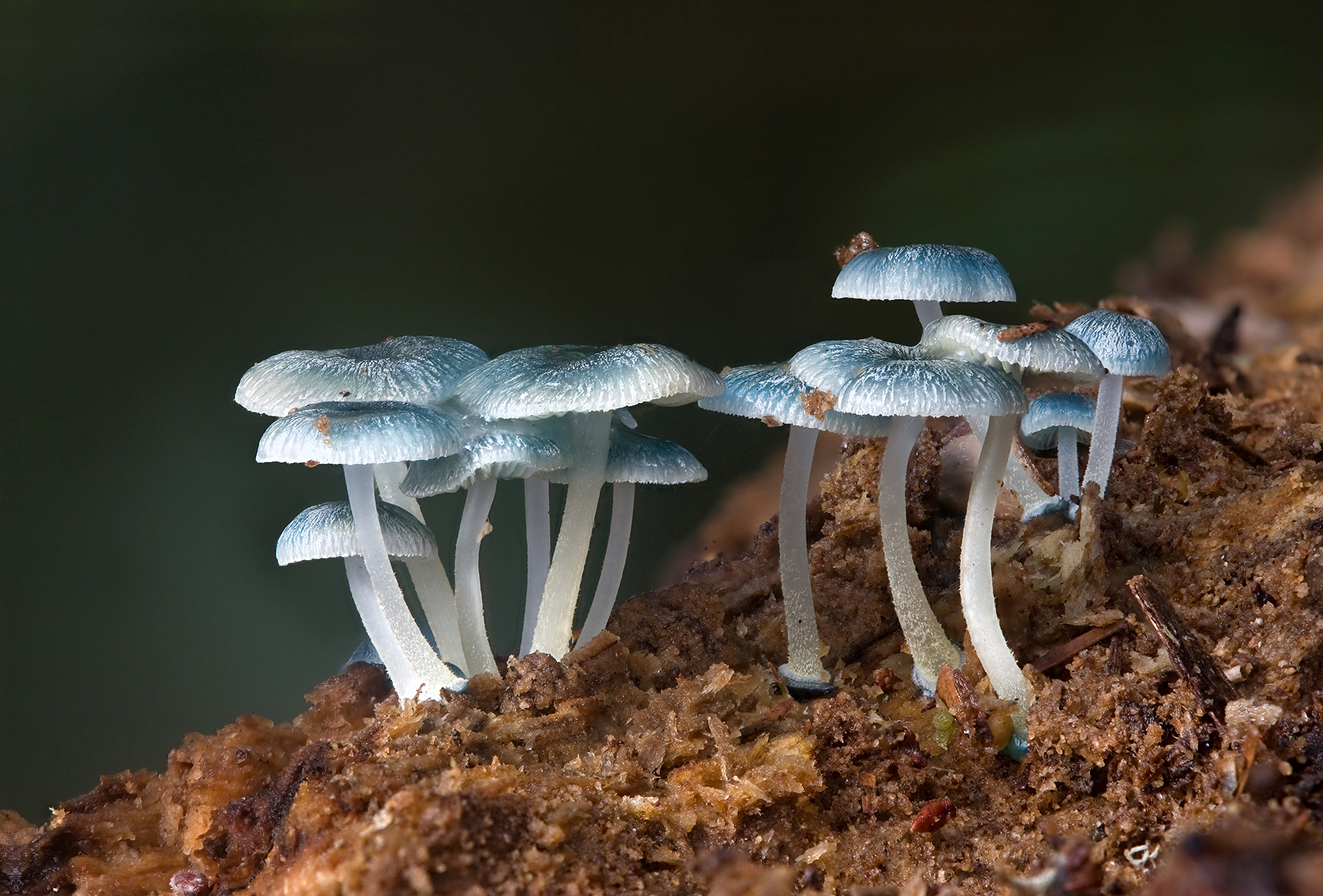
// Image used from http://upload.wikimedia.org/wikipedia/commons/1/16/Mycena_interrupta.jpg
label(
  shift(wd/2,ht/2)*
  graphic("img.jpg"
  ,"width="+string(wd)+"bp"
  +",height="+string(ht)+"bp"
  +",scale="+string(sc)
  ),(0,0)
);
layer();

draw(((0,0)--(wd,ht)/sc),blue+2pt);

int ngrid=10;
int n=(int)(wd/ngrid/sc);
int m=(int)(ht/ngrid/sc);
add(scale(ngrid)*grid(n,m,yellow));

//xlimits(0,wd/sc,crop=true);
//ylimits(0,ht/sc,crop=true);
xaxis( 0,wd/sc,RightTicks(Step=ngrid));
yaxis(0,ht/sc,LeftTicks(Step=ngrid));

pair[] P={
(66,34),
(70,35),
(76,38),
(80,37),
(84,37),
(87,42),
(90,49),
(91,54),
(92,60),
(93,65),
(97,65),
(100,65),
(103,66),
(105,67),
(101,71),
(97,74),
(95,75),
(92,76),
(94,78),
(98,79),
(101,80),
(103,80),
(103,83),
(100,85),
(96,88),
(91,87),
(86,86),
(82,86),
(78,86),
(74,86),
(70,83),
(69,83),
(67,86),
(65,87),
(59,88),
(54,88),
(51,87),
(47,87),
(42,86),
(38,85),
(34,84),
(31,82),
(29,80),
(29,77),
(33,76),
(35,76),
(36,76),
(36,74),
(35,73),
(33,70),
(33,69),
(36,68),
(40,68),
(41,68),
(44,67),
(46,67),
(47,64),
(47,60),
(49,55),
(52,48),
(55,41),
(58,35),
(63,31),
};
guide g=graph(P,operator..)..cycle;
fill(g,white+opacity(0.8));
draw(g,orange+1bp);
\end{asy}
\end{figure}
\end{document}

% To process it with `latexmk`, create file `latexmkrc`:
% 
%     sub asy {return system("asy '$_[0]'");}
%     add_cus_dep("asy","eps",0,"asy");
%     add_cus_dep("asy","pdf",0,"asy");
%     add_cus_dep("asy","tex",0,"asy");
% 
% and run `latexmk -pdf igrid.tex`.
g.kov
  • 21,864
  • 1
  • 58
  • 95
54

To easily get the precise relative positions (which is often quite tedious) and to generate LaTeX code automatically for such example as shown below, you could use the new web-based LaTeX Overlay Generator, which I built for such cases. This is just a small interactive tool, which helps you to find the right locations without using a manual grid-based approach.

Example

LaTeX Code

In the following the source code of a minimal working example generated by the LaTeX Overlay Generator.

\documentclass{article}

% remove "[demo]" if you want include actual image!!!
\usepackage[demo]{graphicx}

\usepackage{tikz}

%%%%%%%%%%%%%%%%%%%%%%%%%%%%%%%%%%%%%%%%%%%%%%%%%%%%%%%%%%%%%%%%%%%%%%
% LaTeX Overlay Generator - Annotated Figures v0.0.1
% Created with http://ff.cx/latex-overlay-generator/
%%%%%%%%%%%%%%%%%%%%%%%%%%%%%%%%%%%%%%%%%%%%%%%%%%%%%%%%%%%%%%%%%%%%%%
%\annotatedFigureBoxCustom{bottom-left}{top-right}{label}{label-position}{box-color}{label-color}{border-color}{text-color}
\newcommand*\annotatedFigureBoxCustom[8]{\draw[#5,thick,rounded corners] (#1) rectangle (#2);\node at (#4) [fill=#6,thick,shape=circle,draw=#7,inner sep=2pt,font=\sffamily,text=#8] {\textbf{#3}};}
%\annotatedFigureBox{bottom-left}{top-right}{label}{label-position}
\newcommand*\annotatedFigureBox[4]{\annotatedFigureBoxCustom{#1}{#2}{#3}{#4}{white}{white}{black}{black}}
\newcommand*\annotatedFigureText[4]{\node[draw=none, anchor=south west, text=#2, inner sep=0, text width=#3\linewidth,font=\sffamily] at (#1){#4};}
\newenvironment {annotatedFigure}[1]{\centering\begin{tikzpicture}
    \node[anchor=south west,inner sep=0] (image) at (0,0) { #1};\begin{scope}[x={(image.south east)},y={(image.north west)}]}{\end{scope}\end{tikzpicture}}
%%%%%%%%%%%%%%%%%%%%%%%%%%%%%%%%%%%%%%%%%%%%%%%%%%%%%%%%%%%%%%%%%%%%%%

\begin{document}

    \begin{figure}[h!t]

        \begin{annotatedFigure}
            {\includegraphics[width=1.0\linewidth]{black-demo.png}}
            \annotatedFigureBox{0.084,0.614}{0.394,0.804}{A}{0.084,0.614}%bl
            \annotatedFigureBox{0.222,0.284}{0.3743,0.4934}{B}{0.3743,0.4934}%tr
            \annotatedFigureBox{0.555,0.784}{0.6815,0.874}{C}{0.555,0.784}%bl
            \annotatedFigureBox{0.557,0.322}{0.8985,0.5269}{D}{0.8985,0.5269}%tr
        \end{annotatedFigure}

        \caption{\textbf{Lorum Ipsum Overview} -- Lorem ipsum dolor amet (A), consetetur (B) elitr, sed diam (C) nonumy eirmod invidunt ut labore (D).}
        \label{fig:teaser}

    \end{figure}

\end{document}
f2cx
  • 881
  • 7
  • 7
54

In meantime there is a new package callouts

In the annotate-environment you define the image width and an annotation scale. If you scale both with the same factor, then you can change the size of the image without loosing the correct relative positions.

Example:

\documentclass[11pt]{scrartcl} % use larger type; default would be 10pt
\usepackage[wby]{callouts}

\begin{document}
  % pic-source: http://upload.wikimedia.org/wikipedia/commons/1/16/Mycena_interrupta.jpg
  \begin{annotate}{\includegraphics[width=1\textwidth]{Mycena_interrupta}}{1}
    % \helpgrid
    \note{0,0}{Center}
    \callout{4,3}{Mushrom}{3,2}
    \arrow{-3,-2.4}{-4.5,-3}
    %And raw tikz
    \draw[very thick,red] (-4,4) rectangle (-3,3);
  \end{annotate}
\end{document}

enter image description here

knut
  • 8,838
21

For simple tasks, such a heavy weapon like tikz is not always necessary. If only simple shapes or text should be added a picture environment is more then enough:

\documentclass{article}

\usepackage{graphicx}

\begin{document}
bla

\begin{picture}(1,0.55038404)%
  \put(0,0){\includegraphics[width=.4\textwidth]{17D2J}}%
  \put(150,50){x axis}%
\end{picture}%

\end{document}

enter image description here

(Example based on https://tex.stackexchange.com/a/347168/36296)

An overview of available shapes inside the picture environment can be found at http://www.weinelt.de/latex/picture.html (unfortunately I only found it in German, does anyone know an English version? Or another overview?)

17

Since 2019, we have the tikz-imagelabels package. I think it has been bundled in TeX Live 2019 onwards.

This package does what the question asks entirely using the standard tikz macros.

Example (taken from the documentation) below. Image source.

    \documentclass{standalone}
     \usepackage{tikz-imagelabels}
 \begin{document}
 \begin{annotationimage}{width=6cm}{pleiades.jpg}
   \draw[annotation left = {Atlas at 0.3}] to (0.11,0.4);
   \draw[annotation left = {Pleione at 0.55}] to (0.11,0.49);
   \draw[annotation left = {Alcyone at 0.8}] to (0.39,0.45);
   \draw[annotation below = {Merope at 0.5}] to (0.58,0.28);
   \draw[annotation right = {Electra at 0.3}] to (0.84,0.45);
   \draw[annotation right = {Caleano at 0.75}] to (0.85,0.64);
   \draw[annotation above = {Maia at 0.4}] to (0.67,0.72);
   \draw[annotation above = {Taygeta at 0.9}] to (0.78,0.82);
   \draw[image label = {M45 at south east}];
 \end{annotationimage}
 \end{document}

Output of tikz-imagelabels example

prash
  • 281