How do I plot coordinates (latitude and longitude pairs) on a geographic map?

Question

I'm attempting for the first time to create a map within Mathematica. In particular, I would like to take an output of points and plot them according to their lat/long values over a geographic map. I have a series of latitude/longitude values like so:

 {{32.6123, -117.041}, {40.6973, -111.9},   {34.0276, -118.046}, 
  {40.8231, -111.986}, {34.0446, -117.94},  {33.7389, -118.024}, 
  {34.122, -118.088},  {37.3881, -122.252}, {44.9325, -122.966}, 
  {32.6029, -117.154}, {44.7165, -123.062}, {37.8475, -122.47}, 
  {32.6833, -117.098}, {44.4881, -122.797}, {37.5687, -122.254}, 
  {45.1645, -122.788}, {47.6077, -122.692}, {44.5727, -122.65},
  {42.3155, -82.9408}, {42.6438, -73.6451}, {48.0426, -122.092}, 
  {48.5371, -122.09},  {45.4599, -122.618}, {48.4816, -122.659}, 
  {42.3398, -70.9843}}

I've tried finding documentation on how I would proceed but I cannot find anything that doesn't assume a certain level of introduction to geospatial data. Does anyone know of a good resource online or is there a simple explanation one can supply here?

score 32 · Accepted Answer · edited Oct 06 '12 at 08:05

data:

latlong = {{32.6123, -117.041}, {40.6973, -111.9}, {34.0276, -118.046}, 
{40.8231, -111.986}, {34.0446, -117.94}, {33.7389, -118.024}, 
{34.122, -118.088}, {37.3881, -122.252}, {44.9325, -122.966},
{32.6029, -117.154}, {44.7165, -123.062}, {37.8475, -122.47}, 
{32.6833, -117.098}, {44.4881, -122.797}, {37.5687, -122.254},
{45.1645, -122.788}, {47.6077, -122.692}, {44.5727, -122.65}, 
{42.3155, -82.9408}, {42.6438, -73.6451}, {48.0426, -122.092},
{48.5371, -122.09}, {45.4599, -122.618}, {48.4816, -122.659}, {42.3398, -70.9843}}

To put the data on latitude-longitude pairs on a map, yo will need to transform your data based on the projection method used by the map.

For example,

 coords = CountryData["UnitedStates", "Coordinates"];

gives the latitude-longitude data for US boundaries.

To use this data to put together a map with a specific projection method (say Mercator), you need to transform your data

 Map[ GeoGridPosition[ GeoPosition[#], "Mercator"][[1]] & , {latlong}, {2}]

which gives

  {{{1.09884, 0.602677}, {1.18857, 0.778879}, {1.0813, 
   0.632239}, {1.18707, 0.781777}, {1.08315, 0.632597}, {1.08169, 
   0.62617}, {1.08057, 0.634228}, {1.00789, 0.704491}, {0.995431, 
   0.879708}, {1.09687, 0.602482}, {0.993756, 0.874393}, {1.00409, 
   0.714614}, {1.09785, 0.604149}, {0.998381, 0.868794}, {1.00786, 
   0.708463}, {0.998538, 0.88544}, {1.00021, 0.947273}, {1.00095, 
   0.870866}, {1.694, 0.816595}, {1.85624, 0.824365}, {1.01069, 
   0.958578}, {1.01072, 0.97155}, {1.0015, 0.892771}, {1.00079, 
   0.970088}, {1.90268, 0.817169}}}

Doing this transformation for both your data and the latitude-longitude data for world countries inside Graphics:

 Graphics[{Red, Point /@ Map[ 
  GeoGridPosition[ GeoPosition[#], 
   "Mercator"][[1]] & , {latlong}, {2}], Gray, 
 Polygon[Map[ GeoGridPosition[ GeoPosition[#], "Mercator"][[1]] & , 
  CountryData[#, "Coordinates"], {2}]] & /@ 
 CountryData["Countries"]}]

you get:

world map and lat-long points

Now I know I can focus on US:

 Graphics[{ Gray, 
 Polygon[Map[ GeoGridPosition[ GeoPosition[#], "Mercator"][[1]] & , 
 CountryData["UnitedStates", "Coordinates"], {2}]], Red, 
 PointSize[.02], Point /@ Map[ 
 GeoGridPosition[ GeoPosition[#], 
   "Mercator"][[1]] & , {latlong}, {2}]}]

to get

us and points

A simpler method avoiding GeoPosition, GeoGridPosition ... etc

Get the coordinates of US:

 coords = CountryData["UnitedStates", "Coordinates"];

and use

 Graphics[{EdgeForm[Black], Polygon[Reverse /@ First[coords]], Red, 
 Point /@ Reverse /@ latlong}]

to get

simpler approach result

How can I have detailed map instead just black, and a contour of the country? — user34018, May 24 '16 at 16:24

score 29 · Answer 2 · answered Feb 21 '12 at 05:47

29

There is nice way to to put your data on rotatable 3D globe. Your data:

centers = {{32.6123, -117.041}, {40.6973, -111.9}, {34.0276, \
-118.046}, {40.8231, -111.986}, {34.0446, -117.94}, {33.7389, \
-118.024}, {34.122, -118.088}, {37.3881, -122.252}, {44.9325, \
-122.966}, {32.6029, -117.154}, {44.7165, -123.062}, {37.8475, \
-122.47}, {32.6833, -117.098}, {44.4881, -122.797}, {37.5687, \
-122.254}, {45.1645, -122.788}, {47.6077, -122.692}, {44.5727, \
-122.65}, {42.3155, -82.9408}, {42.6438, -73.6451}, {48.0426, \
-122.092}, {48.5371, -122.09}, {45.4599, -122.618}, {48.4816, \
-122.659}, {42.3398, -70.9843}};

Function that defines mapping of coordinates onto sphere:

SC[{lat_, lon_}] := r {Cos[lon \[Degree]] Cos[lat \[Degree]], 
Sin[lon  \[Degree]] Cos[lat  \[Degree]], Sin[lat \[Degree]]};

Average Earth radius, countries names, 3D visualization where you can Drag globe to rotate, Hold CTRL and drag to zoom:

r = 6367.5; places = CountryData["Countries"];
Graphics3D[{Opacity[.9], Sphere[{0, 0, 0}, r], 
  Map[Line[Map[SC, CountryData[#, "SchematicCoordinates"], {-2}]] &, 
   places], {Red, PointSize[Medium], Point[SC[#]] & /@ centers}}, 
 Boxed -> False, SphericalRegion -> True, ViewAngle -> .3]

enter image description here

answered Feb 21 '12 at 05:47

Vitaliy Kaurov

73,078
9
204
355

Could you please give some tips on how to extend your method to work with e.g. "SchematicPolygon" instead of coordinates? – István Zachar Mar 18 '12 at 10:57
Dear @VitaliyKaurov I like your solution a lot! One can make the country borders more precise by substituting SchematicCoordinates with FullCoordinates. How can I make the seas and lakes blue and land green or brown? Is there a way to draw a list of lists of coordinates, i.e. plot trajectories of ships? – Leo Apr 06 '20 at 01:01
@Leo please see modern functions – Vitaliy Kaurov Apr 06 '20 at 04:09
@VitaliyKaurov Thank you for your reply. I'm experimenting with GeoGraphics, but I still don't know how to make a rotatable zoomable 3D globe with trajectories of ships. I only managed to create a non-zoomable 2D version with trajectories. What modern method do you think is best for this? – Leo Apr 06 '20 at 22:11
1

@Leo see Texture -> Applications -> Earth Texture Map – Vitaliy Kaurov Apr 07 '20 at 01:45

score 19 · Answer 3 · edited Jun 16 '20 at 09:23

19

Here's a start.

latLngs={{32.6123,-117.041},{40.6973,-111.9},{34.0276,-118.046},
  {40.8231,-111.986},{34.0446,-117.94},{33.7389,-118.024},
  {34.122,-118.088},{37.3881,-122.252},{44.9325,-122.966},
  {32.6029,-117.154},{44.7165,-123.062},{37.8475,-122.47},
  {32.6833,-117.098},{44.4881,-122.797},{37.5687,-122.254},
  {45.1645,-122.788},{47.6077,-122.692},{44.5727,-122.65},
  {42.3155,-82.9408},{42.6438,-73.6451},{48.0426,-122.092},
  {48.5371,-122.09},{45.4599,-122.618},{48.4816,-122.659},
  {42.3398,-70.9843}};
Show[CountryData["UnitedStates",{"Shape", "Equirectangular"}],
  Axes -> True, Epilog ->{PointSize[0.01], Red,
  Point[Reverse /@ latLngs]}]

You can show the points on a natural Mercator projection like so:

toMercator[{lat_, lng_}] := {lng, 
  Log[Abs[Sec[lat*Degree]+Tan[lat*Degree]]]/Degree};
mercPoints = toMercator /@ latLngs;
Show[CountryData["UnitedStates",{"Shape", "Mercator"}],
  Frame-> True, Epilog ->{PointSize[0.01], Red,
  Point[mercPoints]}]

Mathematica graphics

Presumably, there's a built in way to extract the values of from Mercator's (and other) projections, but I don't see how offhand.

edited Jun 16 '20 at 09:23

Community

1

answered Feb 21 '12 at 04:47

Mark McClure

32,469
3
103
161

Interesting, do you share that package on your website? – Vitaliy Kaurov Feb 21 '12 at 07:37
Please review my edit. I think it was necessary to make the package link more visible. I hope you don't mind. – Szabolcs Feb 21 '12 at 11:11
@Vitaliy The package is on my website, as Szabolcs has kindly pointed out. It could be updated. :) – Mark McClure Feb 21 '12 at 22:29
@Szabolcs The edit is certainly an improvement. Thanks. – Mark McClure Feb 21 '12 at 22:30

score 13 · Answer 4 · edited Apr 13 '17 at 12:55

I am a big fan of the Texture functionality... (I'd like to point out, that this is all inspired by graphics/visualisation genius Yu-Sung Chang)

nightEarth = SphericalPlot3D[1, {u, 0, Pi}, {v, 0, 2 Pi},
   PlotPoints -> 50, MaxRecursion -> 0,
   Mesh -> None, TextureCoordinateFunction -> ({#5, 1 - #4} &),
   PlotStyle -> Directive[
      Texture[Import["http://eoimages.gsfc.nasa.gov/images/imagerecords/55000/55167/earth_lights_lrg.jpg"]],   
      Specularity[White, 50]],
   Lighting -> "Neutral", Boxed -> False, Axes -> False, Background -> Gray]

enter image description here

Well this is already gospel:

SC[{lat_, lon_}] := {Cos[(lon + 180) °] Cos[lat °], 
   Sin[(lon + 180) °] Cos[lat °], Sin[lat °]};

Your coordinates:

centers = {{32.6123, -117.041}, {40.6973, -111.9}, {34.0276, \
    -118.046}, {40.8231, -111.986}, {34.0446, -117.94}, {33.7389, \
    -118.024}, {34.122, -118.088}, {37.3881, -122.252}, {44.9325, \
    -122.966}, {32.6029, -117.154}, {44.7165, -123.062}, {37.8475, \
    -122.47}, {32.6833, -117.098}, {44.4881, -122.797}, {37.5687, \
    -122.254}, {45.1645, -122.788}, {47.6077, -122.692}, {44.5727, \
    -122.65}, {42.3155, -82.9408}, {42.6438, -73.6451}, {48.0426, \
    -122.092}, {48.5371, -122.09}, {45.4599, -122.618}, {48.4816, \
    -122.659}, {42.3398, -70.9843}};

and now:

Show[nightEarth, Graphics3D[{Opacity[.9], {Red, PointSize[Medium], 
   Point[SC[#]] & /@ centers}}, Boxed -> False, 
   SphericalRegion -> True, ViewAngle -> .3], ImageSize -> Large]

enter image description here

score 12 · Answer 5 · answered Jun 24 '16 at 18:08

12

Just in case anyone comes across this post in a search, here is a one-liner here for version 10 and after. If latlong is the list from the OP, then you can do this

GeoGraphics[{Red, PointSize[.02], Point@GeoPosition@latlong}]

Mathematica graphics

The input for GeoGraphics is structured like that for Graphics, and you can use a whole host of options

GeoGraphics[{Red, PointSize[.01], Point@GeoPosition@latlong}, 
 GeoRange -> "World", GeoProjection -> "Mollweide", 
 GeoGridLines -> Quantity[5, "AngularDegrees"], 
 GeoBackground -> "ContourMap"]

Mathematica graphics

answered Jun 24 '16 at 18:08

Jason B.

68,381
3
139
286

1

Even shorter is GeoListPlot[GeoPosition /@ latlong]. – Greg Hurst Aug 01 '16 at 21:26
@ChipHurst for some reason, while the first GeoGraphics[{Red, PointSize[.02], Point@GeoPosition@latlong}] command in this answer worked perfectly, I get GeoGraphics::wdata: Unable to download data for ranges {{59.9181103,59.9273349},{30.454744275,30.473620825}} and zoom level 15 from the Wolfram geo server. from your command. – Ruslan Jul 22 '17 at 19:07

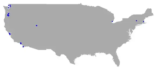
Artes · Answer 6 · 2012-02-21T14:52:29.553

Given latitude/longitude values:

list = {{32.6123, -117.041}, {40.6973, -111.9}, {34.0276, -118.046}, \
        {40.8231, -111.986}, {34.0446, -117.94}, {33.7389, -118.024}, \
        {34.122, -118.088}, {37.3881, -122.252}, {44.9325, -122.966}, \
        {32.6029, -117.154}, {44.7165, -123.062}, {37.8475, -122.47}, \
        {32.6833, -117.098}, {44.4881, -122.797}, {37.5687, -122.254}, \
        {45.1645, -122.788}, {47.6077, -122.692}, {44.5727, -122.65}, \
        {42.3155, -82.9408}, {42.6438, -73.6451}, {48.0426, -122.092}, \
        {48.5371, -122.09}, {45.4599, -122.618}, {48.4816, -122.659}, \
        {42.3398, -70.9843}};

I make a graphics with Tooltip to show coordinates of positions in the list in DMSString {degree, minute, second} format.

Graphics[{Darker[Green], CountryData["UnitedStates", "Polygon"], 
          PointSize[Large], Blue, Tooltip[{PointSize[0.005], Point[Reverse@#]}, 
          DMSString[#]] & /@ list}]

Edit

It would be more useful if we could find two nearest big cities to every specified position in the list. We can fulfill such an expectation with a handy function from Mathematica documentation, like this :

nearLC = Nearest[ CityData[ #, "Coordinates"]
                           -> # & /@  CityData[{Large, "UnitedStates"}]];

Now we can adapt this function to the data we are deal with in order to show with Tooltip two nearest big cities (of population over 100000) for every point :

Graphics[{ Lighter[Gray], CountryData["UnitedStates", "Polygon"], 
           Blue,  Tooltip[{PointSize[0.007], Point[Reverse@#]}, 
           Flatten[ nearLC[#, 2] /. {a_, b_, c_} -> {a, b}]] & /@ list}]

enter image description here

How do I plot coordinates (latitude and longitude pairs) on a geographic map?

6 Answers6

Here's a start.

Linked