Numerically solving Helmholtz equation in 3D for arbitrary shapes

Question

Context

While studying manifold Learning I got interested in finding the eigenvectors of the Laplacian. (also in connection to this problem of solving the heat equation)

Following this and that amazing answer, I am interested in solving this Helmholtz equation in 3D

$ \triangledown^2 u(x,y,z) + k^2u(x,y,z) =0 \quad x,y,z \in \Omega\,, \quad u(x,y,z) = 0 \quad {\rm with}\quad x,y,z \in \partial\Omega $

where $\Omega =$ is some 3D boundary e.g. a ball, an ellipsoid, a regular 3D polygon etc.

---

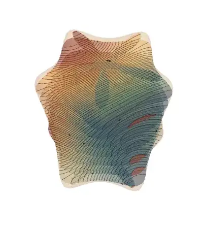
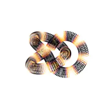
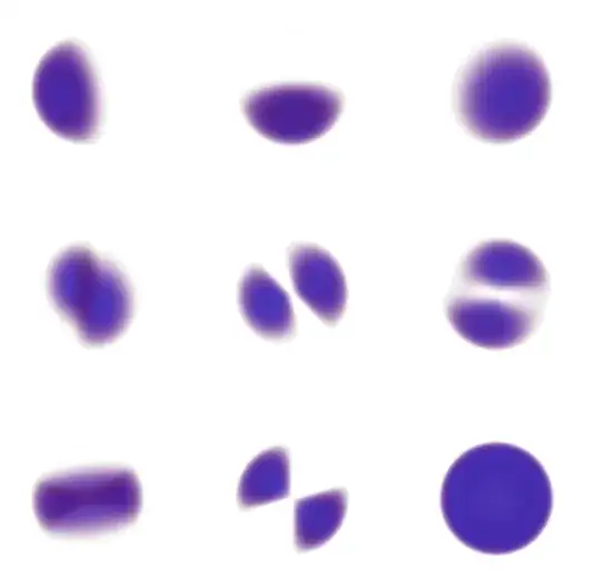
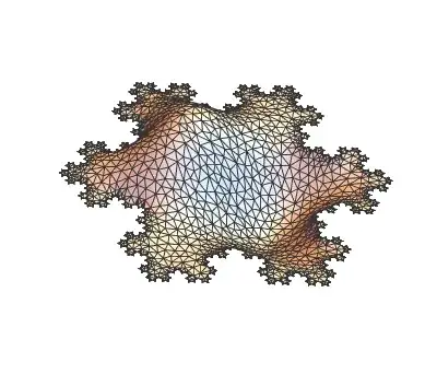
I have played around with the 2D codes provided here to produce these first eigen modes of a snowflake (again beautiful code!):

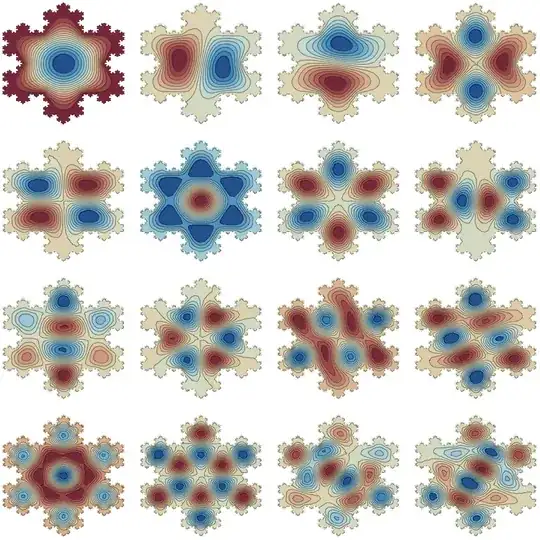
They look like this and are super-cool!

but I would like to generalize their answer to 3D.

---

Question

How would one proceed in 3D, given that we have a 2D solution working?

---

Cheeky Attempt

I have modified slightly Mark McClure's code to make it 3D savvy, but I am no expert in this field

Needs["NDSolve`FEM`"];
helmholzSolve3D[g_, numEigenToCompute_Integer, 
  opts : OptionsPattern[]] := 
 Module[{u, x, y, z, t, pde, dirichletCondition, mesh, boundaryMesh, 
   nr, state, femdata, initBCs, methodData, initCoeffs, vd, sd, 
   discretePDE, discreteBCs, load, stiffness, damping, pos, nDiri, 
   numEigen, res, eigenValues, eigenVectors, 
   evIF},(*Discretize the region*)
  If[Head[g] === ImplicitRegion || Head[g] === ParametricRegion, 
   mesh = ToElementMesh[DiscretizeRegion[g], opts], 
   mesh = ToElementMesh[DiscretizeGraphics[g], opts]];
  boundaryMesh = ToBoundaryMesh[mesh];
  (*Set up the PDE and boundary condition*)
  pde = D[u[t, x, y, z], t] - Laplacian[u[t, x, y, z], {x, y, z}] + 
     u[t, x, y, z] == 0;
  dirichletCondition = DirichletCondition[u[t, x, y, z] == 0, True];
  (*Pre-process the equations to obtain the FiniteElementData in \
StateData*)nr = ToNumericalRegion[mesh];
  {state} = 
   NDSolve`ProcessEquations[{pde, dirichletCondition, 
     u[0, x, y, z] == 0}, u, {t, 0, 1}, Element[{x, y, z}, nr]];
  femdata = state["FiniteElementData"];
  initBCs = femdata["BoundaryConditionData"];
  methodData = femdata["FEMMethodData"];
  initCoeffs = femdata["PDECoefficientData"];
  (*Set up the solution*)vd = methodData["VariableData"];
  sd = NDSolve`SolutionData[{"Space" -> nr, "Time" -> 0.}];
  (*Discretize the PDE and boundary conditions*)
  discretePDE = DiscretizePDE[initCoeffs, methodData, sd];
  discreteBCs = 
   DiscretizeBoundaryConditions[initBCs, methodData, sd];
  (*Extract the relevant matrices and deploy the boundary conditions*)
  load = discretePDE["LoadVector"];
  stiffness = discretePDE["StiffnessMatrix"];
  damping = discretePDE["DampingMatrix"];
  DeployBoundaryConditions[{load, stiffness, damping}, discreteBCs];
  (*Set the number of eigenvalues ignoring the Dirichlet positions*)
  pos = discreteBCs["DirichletMatrix"]["NonzeroPositions"][[All, 2]];
  nDiri = Length[pos];
  numEigen = numEigenToCompute + nDiri;
  (*Solve the eigensystem*)
  res = Eigensystem[{stiffness, damping}, -numEigen];
  res = Reverse /@ res;
  eigenValues = res[[1, nDiri + 1 ;; Abs[numEigen]]];
  eigenVectors = res[[2, nDiri + 1 ;; Abs[numEigen]]];
  evIF = ElementMeshInterpolation[{mesh}, #] & /@ eigenVectors;
  (*Return the relevant information*){eigenValues, evIF, mesh}]

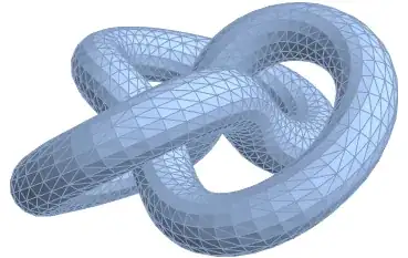
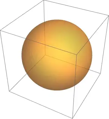
If I then define a 3D boundary

   Ω = ImplicitRegion[0 <= x^2 + y^2 + z^2 <= 1, {x, y, z}];
     RegionPlot3D[Ω, PlotStyle -> Opacity[0.5]]

Naively this should give me the eigenmode:

{ev, if, mesh} = helmholzSolve3D[Ω, 1];
ev

but it actually crashes the kernel Mathematica (10.0.2).

Could anyone confirm this as a first step?

NB: Please do not loose sleep over this problem as it is mostly driven by curiosity :-)

PS: On the other hand I personally think this stuff is truly one of the best new useful features of Mathematica 10!

Answer 1

Version 11 has both symbolic and numeric eigensolvers, see here for an overview

Here is a slightly different way to do it. We write a function that converts any PDE (1D/2D/3D) into discretized system matices:

Needs["NDSolve`FEM`"]
PDEtoMatrix[{pde_, Γ___}, u_, r__, 
  o : OptionsPattern[NDSolve`ProcessEquations]] := 
 Module[{ndstate, feData, sd, bcData, methodData, pdeData},
  {ndstate} =
   NDSolve`ProcessEquations[Flatten[{pde, Γ}], u, 
    Sequence @@ {r}, o];
  sd = ndstate["SolutionData"][[1]];
  feData = ndstate["FiniteElementData"];
  pdeData = feData["PDECoefficientData"];
  bcData = feData["BoundaryConditionData"];
  methodData = feData["FEMMethodData"];
  {DiscretizePDE[pdeData, methodData, sd], 
   DiscretizeBoundaryConditions[bcData, methodData, sd], sd, 
   methodData}
  ]

Example 1: An eigensolver is then something like this:

     {dPDE, dBC, sd, md} = 
  PDEtoMatrix[{D[u[t, x, y], t] == Laplacian[u[t, x, y], {x, y}], 
    u[0, x, y] == 0, DirichletCondition[u[t, x, y] == 0, True]}, 
   u, {t, 0, 1}, {x, y} ∈ Rectangle[]];
l = dPDE["LoadVector"];
s = dPDE["StiffnessMatrix"];
d = dPDE["DampingMatrix"];
constraintMethod = "Remove";
DeployBoundaryConditions[{l, s, d}, dBC, 
  "ConstraintMethod" -> "Remove"];
First[es = Reverse /@ Eigensystem[{s, d}, -4, Method -> "Arnoldi"]]

If[constraintMethod === "Remove", 
  es[[2]] = 
    NDSolve`FEM`DirichletValueReinsertion[#, dBC] & /@ es[[2]];];

ifs = ElementMeshInterpolation[sd, #] & /@ es[[2]];
mesh = ifs[[2]]["ElementMesh"];
ContourPlot[#[x, y], {x, y} ∈ mesh, Frame -> False, 
   ColorFunction -> ColorData["RedBlueTones"]] & /@ ifs

This can be encapsulated as follows:

Helmholtz2D[bdry_, order_] :=
 Module[{dPDE, dBC, sd, md, l, s, d, ifs, es, mesh, 
   constraintMethod},
  {dPDE, dBC, sd, md} = 
   PDEtoMatrix[{D[u[t, x, y], t] == Laplacian[u[t, x, y], {x, y}], 
     u[0, x, y] == 0, DirichletCondition[u[t, x, y] == 0, True]}, 
    u, {t, 0, 1}, {x, y} ∈ bdry];
  l = dPDE["LoadVector"];
  s = dPDE["StiffnessMatrix"];
  d = dPDE["DampingMatrix"];
  constraintMethod = "Remove";
  DeployBoundaryConditions[{l, s, d}, dBC, 
   "ConstraintMethod" -> "Remove"];
  First[es = Reverse /@ Eigensystem[{s, d}, -order, Method -> "Arnoldi"]]
   If[constraintMethod === "Remove", 
    es[[2]] = 
      NDSolve`FEM`DirichletValueReinsertion[#, dBC] & /@ es[[2]];];
  ifs = ElementMeshInterpolation[sd, #] & /@ es[[2]];
  mesh = ifs[[2]]["ElementMesh"];
  {es, ifs, mesh}
  ]

Example 2: The the remaining problem in the question can then be solved like this:

RR = ImplicitRegion[
   x^6 - 5 x^4 y z + 3 x^4 y^2 + 10 x^2 y^3 z + 3 x^2 y^4 - y^5 z + 
     y^6 + z^6 <= 
    1, {{x, -1.25, 1.25}, {y, -1.25, 1.25}, {z, -1.25, 1.25}}];
mesh = ToElementMesh[RR, 
  "BoundaryMeshGenerator" -> {"RegionPlot", "SamplePoints" -> 31}]

mesh["Wireframe"]

This creates a second order mesh with about 80T tets and 140T nodes. To discretize the PDE we use:

AbsoluteTiming[{dPDE, dBC, sd, md} = 
   PDEtoMatrix[{D[u[t, x, y, z], t] == 
      Laplacian[u[t, x, y, z], {x, y, z}], u[0, x, y, z] == 0, 
     DirichletCondition[u[t, x, y, z] == 0, True]}, 
    u, {t, 0, 1}, {x, y, z} ∈ mesh];
 ]
{6.24463, Null}

Get the eigenvalues and vectors:

l = dPDE["LoadVector"];
s = dPDE["StiffnessMatrix"];
d = dPDE["DampingMatrix"];
DeployBoundaryConditions[{l, s, d}, dBC, 
  "ConstraintMethod" -> "Remove"];
AbsoluteTiming[
 First[es = Reverse /@ Eigensystem[{s, d}, -4, Method -> "Arnoldi"]]
 ]
{13.484131`, {8.396796994677874`, 16.044484716974942`, 
  17.453692912770126`, 17.45703443132916`}}

Post process / visualize:

ifs = ElementMeshInterpolation[sd, #, 
     "ExtrapolationHandler" -> {(Indeterminate &),
              "WarningMessage" -> False}] & /@ es[[2]];

Generate slices of the eigenfunctions in the region:

ctrs = Range @@ 
   Join[mm = 
     MinMax[ifs[[2]]["ValuesOnGrid"]], {Abs[Subtract @@ mm]/50}];
levels = Range[-1.25, 1.25, 0.25];
res = ContourPlot[
     ifs[[2]][x, y, #], {x, -1.25, 1.25}, {y, -1.25, 1.25}, 
     Frame -> False, ColorFunction -> ColorData["RedBlueTones"], 
     Contours -> ctrs] & /@ levels;
Show[{
  RegionPlot3D[RR, PlotPoints -> 31, 
   PlotStyle -> Directive[Opacity[0.25]]],
  Graphics3D[{Opacity[0.25], Flatten[MapThread[
      Function[{gr, l}, 
       Cases[gr, _GraphicsComplex] /. 
        GraphicsComplex[coords_, rest__] :> 
         GraphicsComplex[
          Join[coords, ConstantArray[{l}, {Length[coords]}], 2], 
          rest]],
      {res, levels}]]}]
  }, Boxed -> False, Background -> Gray]

Example 3: As a self contained example, let us encapsulate the Helmholtz solver

 Helmholtz3D[bdry_, order_] :=   
     Module[{dPDE, dBC, sd, md, l, s, d, ifs, es, mesh, 
       constraintMethod},
      {dPDE, dBC, sd, md} = 
       PDEtoMatrix[{D[u[t, x, y, z], t] == 
          Laplacian[u[t, x, y, z], {x, y, z}], u[0, x, y, z] == 0, 
         DirichletCondition[u[t, x, y, z] == 0, True]}, 
        u, {t, 0, 1}, {x, y, z} ∈ bdry];
      l = dPDE["LoadVector"];
      s = dPDE["StiffnessMatrix"];
      d = dPDE["DampingMatrix"];
      constraintMethod = "Remove";
      DeployBoundaryConditions[{l, s, d}, dBC, 
       "ConstraintMethod" -> "Remove"];
      First[es = Reverse /@ Eigensystem[{s, d}, -4, Method -> "Arnoldi"]]
       If[constraintMethod === "Remove", 
        es[[2]] = 
          NDSolve`FEM`DirichletValueReinsertion[#, dBC] & /@ es[[2]];];
      ifs = ElementMeshInterpolation[sd, #] & /@ es[[2]];
      mesh = ifs[[2]]["ElementMesh"];
      {es, ifs, mesh}
      ]

and consider

RR = ImplicitRegion[
  x^4 + y^4 + z^4 < 1, {{x, -1, 1}, {y, -1, 1}, {z, -1, 1}}]

{es, ifs, mesh} = Helmholtz3D[RR, nm=4];
mm = MinMax[ifs[[nm]]["ValuesOnGrid"]];
Map[{Opacity[0.4], PointSize[0.01], 
ColorData["Heat"][0.3 + 1/mm[[2]] ifs[[nm]][Sequence @@ #]], 
Point[#]} &, mesh["Coordinates"]] // 
 Graphics3D[#, Boxed -> False] &

Example 4 Eigen modes on 3D Knot

Needs["NDSolve`FEM`"]
f[t_] := With[{s = 3 t/2}, {(2 + Cos[s]) Cos[t], (2 + Cos[s]) Sin[t], 
    Sin[s]} - {2, 0, 0}]
v1[t_] := Cross[f'[t], {0, 0, 1}] // Normalize
v2[t_] := Cross[f'[t], v1[t]] // Normalize
g[t_, θ_] := 
 f[t] + (Cos[θ] v1[t] + Sin[θ] v2[t])/2
gr = ParametricPlot3D[
   Evaluate@g[t, θ], {t, 0, 4 Pi}, {θ, 0, 2 Pi}, 
   Mesh -> None, MaxRecursion -> 4, Boxed -> False, Axes -> False];
tscale = 4; θscale = 0.5;(*scale roughly proportional to \
speeds*)dom = 
 ToElementMesh[
  FullRegion[2], {{0, tscale}, {0, θscale}},(*domain*)
  MaxCellMeasure -> {"Area" -> 0.001}];
coords = g[4 Pi #1/tscale, 2 Pi #2/θscale] & @@@ 
  dom["Coordinates"];(*apply g*)bmesh2 = 
 ToBoundaryMesh["Coordinates" -> coords, 
  "BoundaryElements" -> dom["MeshElements"]];
emesh2 = ToElementMesh@bmesh2;
RR = MeshRegion@emesh2

{es, ifs, mesh} = Helmholtz3D[RR, nm = 4];

then

mm = MinMax[ifs[[nm]]["ValuesOnGrid"]];
Map[{Opacity[0.4], PointSize[0.01], 
    ColorData["Heat"][0.3 + 1/mm[[2]] ifs[[nm]][Sequence @@ #]],
    Point[#]} &, emesh2["Coordinates"]] // 
 Graphics3D[#, Boxed -> False] &

Answer 2

This slightly modified function

 Needs["NDSolve`FEM`"];
    helmholzSolve3D[g_, numEigenToCompute_Integer, 
      opts : OptionsPattern[]] := 
     Module[{u, x, y, z, t, pde, dirichletCondition, mesh, boundaryMesh, 
       nr, state, femdata, initBCs, methodData, initCoeffs, vd, sd, 
       discretePDE, discreteBCs, load, stiffness, damping, pos, nDiri, 
       numEigen, res, eigenValues, eigenVectors, 
       evIF},(*Discretize the region*)
      If[Head[g] === ImplicitRegion || Head[g] === ParametricRegion, 
       mesh = ToElementMesh[DiscretizeRegion[g,opts], opts], 
       mesh = ToElementMesh[DiscretizeGraphics[g,opts], opts]];
      boundaryMesh = ToBoundaryMesh[mesh];
      (*Set up the PDE and boundary condition*)
      pde = D[u[t, x, y, z], t] - Laplacian[u[t, x, y, z], {x, y, z}] + 
         u[t, x, y, z] == 0;
      dirichletCondition = DirichletCondition[u[t, x, y, z] == 0, True];
      (*Pre-process the equations to obtain the FiniteElementData in \
    StateData*)nr = ToNumericalRegion[mesh];
      {state} = 
       NDSolve`ProcessEquations[{pde, dirichletCondition, 
         u[0, x, y, z] == 0}, u, {t, 0, 1}, Element[{x, y, z}, nr]];
      femdata = state["FiniteElementData"];
      initBCs = femdata["BoundaryConditionData"];
      methodData = femdata["FEMMethodData"];
      initCoeffs = femdata["PDECoefficientData"];
      (*Set up the solution*)vd = methodData["VariableData"];
      sd = NDSolve`SolutionData[{"Space" -> nr, "Time" -> 0.}];
      (*Discretize the PDE and boundary conditions*)
      discretePDE = DiscretizePDE[initCoeffs, methodData, sd];
      discreteBCs = 
       DiscretizeBoundaryConditions[initBCs, methodData, sd];
      (*Extract the relevant matrices and deploy the boundary conditions*)
      load = discretePDE["LoadVector"];
      stiffness = discretePDE["StiffnessMatrix"];
      damping = discretePDE["DampingMatrix"];
      DeployBoundaryConditions[{load, stiffness, damping}, discreteBCs];
      (*Set the number of eigenvalues ignoring the Dirichlet positions*)
      pos = discreteBCs["DirichletMatrix"]["NonzeroPositions"][[All, 2]];
      nDiri = Length[pos];
      numEigen = numEigenToCompute + nDiri;
      (*Solve the eigensystem*)
      res = Eigensystem[{stiffness, damping}, -numEigen];
      res = Reverse /@ res;
      eigenValues = res[[1, nDiri + 1 ;; Abs[numEigen]]];
      eigenVectors = res[[2, nDiri + 1 ;; Abs[numEigen]]];
      evIF = ElementMeshInterpolation[{mesh}, #] & /@ eigenVectors;
      (*Return the relevant information*){eigenValues, evIF, mesh}]

works;

For a cuboid

 {ev, if, mesh} =  helmholzSolve3D[Cuboid[], 4, MaxCellMeasure -> .05,  AccuracyGoal -> 2];
 ev

(* {38.2695,85.4791} *)

so that if we look at cross sections

Table[ContourPlot[if[[i]][x, y, 0.5], {x, 0, 1}, {y, 0, 1}],
{i, 4}] // Partition[#, 2] & // GraphicsGrid

or in 3D

Table[ContourPlot3D[if[[i]][x, y, z], {x, 0, 1}, {y, 0, 1}, {z, 0, 1},
 Contours -> {-1/4, 1/4}],{i,4}]

We can the boost up the resolution and look at higher order eigenmodes

{ev, if, mesh} = 
 helmholzSolve3D[Cuboid[], 12, MaxCellMeasure -> 0.0025, 
  "MaxBoundaryCellMeasure" -> 0.025]; Table[
 ContourPlot[if[[i]][x, y, 0.5], {x, 0, 1}, {y, 0, 1},
  Frame -> False, ColorFunction -> ColorData["RedBlueTones"]],

Table[Image3D[
    Table[if[[i]][x, y, z], {x, 0, 1, 0.025}, {y, 0, 1, 0.025}, {z, 0,
       1, 0.025}], ColorFunction -> "RainbowOpacity"],
   {i, 1, 9}] // Partition[#, 3] & // GraphicsGrid

For a ball

{ev, if, mesh} = helmholzSolve3D[Ball[], 12, MaxCellMeasure -> 0.025];

Then

  Table[ContourPlot[if[[i]][x, y, 0.], {x, -1, 1}, {y, -1, 1},
    RegionFunction -> Function[{x, y}, Sqrt[x^2 + y^2] <= 1],
    Frame -> False, Axes -> False, 
    ColorFunction -> ColorData["RedBlueTones"]],
   {i, 12}] // Partition[#, 2] & // GraphicsGrid

Table[Image3D[
    Table[If[x^2 + y^2 + z^2 < 1, if[[i]][x, y, z], 0], {x, -1, 1, 
      0.025}, {y, -1, 1, 0.025}, {z, -1, 1, 0.025}], 
    ColorFunction -> "RainbowOpacity"],
   {i, 2, 11}] // Partition[#, 3] & // GraphicsGrid

It also works for, say a cone

  {ev, if, mesh} = helmholzSolve3D[Cone[], 4, MaxCellMeasure -> 0.25]

Ellipsoid

{ev, if, mesh} = 
 helmholzSolve3D[Ellipsoid[{0, 0, 0}, {1, 2, 3}], 4, 
  MaxCellMeasure -> 0.025]

Table[ContourPlot[if[[i]][x, y, 0.1], {x, -1, 1}, {y, -2, 2}, 
  RegionFunction -> Function[{x, y}, x^2/1 + y^2/2^2 < 1],
  Frame -> False, ColorFunction -> ColorData["RedBlueTones"], 
  AspectRatio -> 1/2],
 {i, 1, 4}]

Arbitrary boundary

It should work on say this cool boundary

RR = ImplicitRegion[
   x^6 - 5 x^4 y z + 3 x^4 y^2 + 10 x^2 y^3 z + 3 x^2 y^4 - y^5 z + 
     y^6 + z^6 <= 1, {x, y, z}];

But unfortunately not with mathematica 10.0.2 because of this bug

If someone with 10.1 care to try this?

{ev, if, mesh} = helmholzSolve3D[RR, 4, MaxCellMeasure -> 0.25]

I get

MathKernel: /Jenkins/workspace/Component.TetGenLink.Linux-x86-64.10.0/Mathematica/Paclets/TetGenLink/CSource/TetGen/tetgen.cxx:19959: tetgenmesh::interresult tetgenmesh::scoutsubface(tetgenmesh::face*, tetgenmesh::triface*, int): Assertion `checksh.sh == dummysh' failed.

Update

with Mathematica 10.2 It just crashes the kernel.