34

I wonder what is the best practice for interpolating curves? Usually, I'm using BSplineCurve and adjusting SplineWeights so it would fit better (and assigning more weight around the sharp edges to drag the curve closer to it). Or if I can guess what formula describes the points, I use FindFit. But often, I can't guess the formula and adjusting weights is very tedious, so it's easier to just manually draw the curve along the points. So what is the best way to join points in Mathematica?

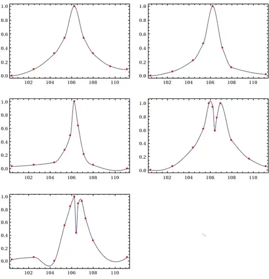
Consider these five sets of points describing five resonance curves for example:

 data = {{{100.434, 0.}, {102.461, 0.0909091}, {104.392, 0.318182}, {105.321, 0.545455},
          {106.226, 1.}, {107.108, 0.545455}, {107.965, 0.318182}, {109.608, 0.136364},
          {111.154, 0.0909091}},
         {{100.434, 0.}, {102.461, 0.06}, {104.392, 0.22}, {105.321, 0.46}, {106.226, 1.},
          {107.108, 0.4}, {107.965, 0.12}, {111.154, 0.02}, {113.958, 0.}},
         {{100.434, 0.030303}, {102.461, 0.0505051}, {104.392, 0.0909091},
          {105.321, 0.272727}, {105.867, 0.494949}, {106.226, 1.}, {106.582, 0.636364},
          {107.108, 0.212121}, {107.965, 0.0505051}, {111.154, 0.}},
         {{100.434, 0.}, {102.461, 0.0555556}, {104.392, 0.333333}, {105.321, 0.611111},
          {105.867, 1.}, {106.226, 0.944444}, {106.405, 0.583333}, {106.582, 0.777778},
          {106.933, 1.}, {107.965, 0.444444}, {109.608, 0.166667}, {111.154, 0.0555556}},
         {{100.434, 0.0188679}, {102.461, 0.0566038}, {104.392, 0.}, {105.321, 0.54717},
          {105.867, 0.849057}, {106.226, 1.}, {106.405, 0.433962}, {106.582, 0.886792},
          {106.933, 0.924528}, {107.281, 0.660377}, {107.965, 0.320755},
          {111.154, 0.0566038}}}
J. M.'s missing motivation
  • 124,525
  • 11
  • 401
  • 574
swish
  • 7,881
  • 26
  • 48
  • Are you aware of 
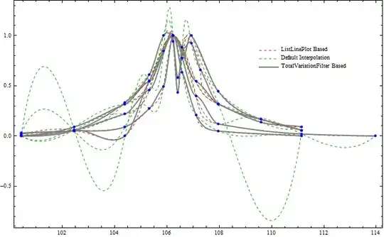
Interpolation[]? – VLC Nov 02 '12 at 16:53
  • @VLC It produces very not smooth curve. – swish Nov 02 '12 at 17:00
  • @VLC With Method -> "Spline" it produces quite smooth curve but still not like I would join it manually. Is there a better way? – swish Nov 02 '12 at 17:07
  • @PlatoManiac As I said it's five functions. – swish Nov 02 '12 at 17:16
  • @swish Show[ListLinePlot[#, InterpolationOrder -> 3, Method -> "Spline", PlotRange -> All, PlotStyle -> Hue[RandomReal[]], Frame -> True, Axes -> None] & /@ data, Epilog -> {Red, PointSize[Medium], Point[Flatten[data, 1]]}] how do you find the interpolation? I guess this is quite a nice interpolation as the functions are at least twice differentiable. – PlatoManiac Nov 02 '12 at 17:29
  • @PlatoManiac It makes a curve go exactly through the points, that can create some ugly bumps sometimes. – swish Nov 02 '12 at 17:48
  • @swish interpolation by definition will go through the given data points. For a smoother behavior you need to control the derivatives at those bumpy points then. – PlatoManiac Nov 02 '12 at 17:55
  • would this help?http://mathematica.stackexchange.com/a/10997/1089 – chris Nov 02 '12 at 18:07
  • @PlatoManiac how come I get something slightly different when I do ff = Interpolation[#, Method -> "Spline", InterpolationOrder -> 3] & /@ data; Plot[#[x] & /@ ff // Release, {x, 101, 111}, Epilog -> {Red, PointSize[Medium], Point[Flatten[data, 1]]}] – chris Nov 02 '12 at 18:11
  • Let's clarify your requirements, shall we? Do you need your interpolant's first and second derivatives to be continuous as well the interpolant itself, or are you fine with just the interpolant and its derivative being continuous? – J. M.'s missing motivation Nov 02 '12 at 21:24
  • Great answers so far. Maybe there will be some method to make a curve don't go directly through the points with second derivative not changing sign very often. – swish Nov 03 '12 at 16:38

2 Answers2

46

So, what is the best way to join points in Mathematica?

There is no one "best way" (not only in Mathematica, but in general); an interpolation scheme that behaves nicely for data set A might be a crapshoot when applied to data set B. It depends on the configuration of your points, and impositions you have on the interpolant (e.g. $C^1$/$C^2$ continuity, preservation of monotonicity/convexity, etc.), with these impositions not always being achievable all at the same time.

Having said this, if you're fine with a $C^1$ interpolant (interpolant and first derivative are continuous), one possibility is to use Akima interpolation. It is not always guaranteed to preserve shape (unless your points are specially configured), but at least for your data set, it does a decent job:

AkimaInterpolation[data_] := Module[{dy}, dy = #2/#1 & @@@ Differences[data];
          Interpolation[Transpose[{List /@ data[[All, 1]], data[[All, -1]], 
                        With[{wp = Abs[#4 - #3], wm = Abs[#2 - #1]}, 
                             If[wp + wm == 0, (#2 + #3)/2, (wp #2 + wm #3)/(wp + wm)]] &
                        @@@ Partition[ArrayPad[dy, 2, "Extrapolated"], 4, 1]}], 
                        InterpolationOrder -> 3, Method -> "Hermite"]]

MapIndexed[(h[#2[[1]]] = AkimaInterpolation[#1]) &, data];

Partition[Table[Plot[{h[k][u]}, {u, 100.434, 111.154}, Axes -> None, 
                     Epilog -> {Directive[Red, AbsolutePointSize[4]], Point[data[[k]]]},
                     Frame -> True, PlotRange -> All],
                {k, 5}], 2, 2, 1, SpanFromBoth] // GraphicsGrid

Akima interpolants for resonance curves

Note that in the fifth plot, the Akima interpolant has a slight wiggle before hitting the third point; this, as I said, is due to the fact that Akima's scheme does not guarantee that it will respect the monotonicity of the data. If you want something that fits a bit more snugly, one scheme you can use is Steffen interpolation, which is also a $C^1$ interpolation method:

SteffenEnds[h1_, h2_, d1_, d2_] :=
       With[{p = d1 + h1 (d1 - d2)/(h1 + h2)}, (Sign[p] + Sign[d1]) Min[Abs[p]/2, Abs[d1]]]

SteffenInterpolation[data_?MatrixQ] := Module[{del, h, pp, xa, ya},
  {xa, ya} = Transpose[data]; del = Differences[ya]/(h = Differences[xa]);
  pp = MapThread[Reverse[#1].#2 &, Map[Partition[#, 2, 1] &, {h, del}]]/
       ListConvolve[{1, 1}, h];
  Interpolation[Transpose[{List /@ xa, ya, 
                Join[{SteffenEnds[h[[1]], h[[2]], del[[1]], del[[2]]]},
                     ListConvolve[{1, 1}, 2 UnitStep[del] - 1] *
                     MapThread[Min, {Partition[Abs[del], 2, 1], Abs[pp]/2}],
                     {SteffenEnds[h[[-1]], h[[-2]], del[[-1]], del[[-2]]]}]}], 
                InterpolationOrder -> 3, Method -> "Hermite"]]

MapIndexed[(w[#2[[1]]] = SteffenInterpolation[#1]) &, data]

Partition[Table[Plot[{w[k][u]}, {u, 100.434, 111.154}, Axes -> None, 
                     Epilog -> {Directive[Red, AbsolutePointSize[4]], Point[data[[k]]]},
                     Frame -> True, PlotRange -> All],
                {k, 5}], 2, 2, 1, SpanFromBoth] // GraphicsGrid

Steffen interpolants for resonance curves

Note that the interpolants from Steffen's method are a lot less wiggly, though the interpolant turns more sharply at its extrema. The advantage of using Steffen is that it is guaranteed to preserve the shape of the data, which might be more important than a smooth turn in some applications.

My point, now, is that sometimes, one must try a number of interpolation schemes to see what is most suitable for the data at hand, for which plotting the interpolant along with the data it is interpolating is paramount.

J. M.'s missing motivation
  • 124,525
  • 11
  • 401
  • 574
  • This is a fantastic answer! Thank you. – Gleno Sep 29 '13 at 14:28
  • Well, I did my best. :) i'll note that the "Akima interpolation" implemented here is his older method; he has a newer method, but I haven't gotten around to writing a Mathematica implementation. – J. M.'s missing motivation May 02 '15 at 03:19
  • It's been almost two years now, and I have to thank you again - because this answer has been very influential on what I've been using (Akima, and Steffen interpolations mostly). I wrote some C code for it that my employer is using now. I'll check out this newer method as well, thanks. :) – Gleno May 02 '15 at 23:21
24

May not turn out to be a very general method but here I will adapt the Interpolation function of MMA in a way so that smoother result can be obtained for your specific data set.

Interpolation vs. ListLinePlot

First lets see how the default Interpolation behaves compared to the interpolating function used when we call ListLinePlot with same interpolation specification. We use Method-> "Spline" in both cases and vary the InterpolationOrder from 1 to 4.

GraphicsGrid[{
 Table[ff =Interpolation[#, Method -> "Spline", InterpolationOrder -> i] & /@data;
       Plot[#[x] & /@ ff // Release, {x, 101, 111},Frame -> None, Axes -> True,
       Epilog -> {Red, PointSize[Medium], Point[Flatten[data, 1]]}],
      {i, 1, 4}],
 Table[Show[
       ListLinePlot[#, InterpolationOrder -> i, Method -> "Spline",PlotRange -> All,
       PlotStyle -> Hue[RandomReal[]],Frame -> None, Axes -> True] & /@ data, 
       Epilog -> {Red, PointSize[Medium], Point[Flatten[data, 1]]}],
      {i,1, 4}]
  }, Frame -> All, AspectRatio -> .5]

enter image description here

The plots in the first column are using default Interpolation function and they starts to oscillate quite naturally as from left to right higher order splines are used. We notice the plots using ListLinePlot are definitely more similar to what the OP is aspiring to achieve. We can get a less bumpy interpolation that still belongs to the $C^{3}(X)$ space of three times differentiable functions as follows.

Function I (ListPlotInterpolation):

Options[ListPlotInterpolation] = {InterpolationOrder -> 3,Method -> Automatic};
ListPlotInterpolation[data_, OptionsPattern[]] := Module[{pic, pts},
      pic = ListLinePlot[data, Method -> OptionValue[Method],
            InterpolationOrder -> OptionValue[InterpolationOrder],PlotRange -> All];
      Interpolation[First@Cases[pic, Line[pts : {{_, _} ..}] -> pts, Infinity], 
             InterpolationOrder -> OptionValue[InterpolationOrder], 
             Method -> OptionValue[Method]
       ]
 ];

Usage:

ListPlotInterpolation[data[[5]], Method -> "Spline",InterpolationOrder -> 3]

InterpolatingFunction[{{100.434,111.154}},<>]

In the following pic the plot in the left shows interpolation of the five given data sets using the above function and all of them are indeed less oscillating than the default Interpolation results with same options at the right . enter image description here

Taming the derivatives!

We can make the above situation a little better by taking the design advantage of the magic function Interpolation. We can always specify the derivatives numerically at the grid points to control the bumpiness of the interpolating function. We will first use ListPlotInterpolation'[] to estimate the derivative at the given grid points. Then we use the TotalVariationFilter to regularize the discrete gradient further on.

Function II (InterpolationReduced):

Options[InterpolationReduced] = {InterpolationOrder -> 3, Method -> Automatic};
InterpolationReduced[data_, OptionsPattern[]] := 
    Module[{fun, coords, value},
        fun = ListPlotInterpolation[data, Method -> OptionValue[Method], 
        InterpolationOrder -> OptionValue[InterpolationOrder]];
        coords = data // Transpose // First;
        value = Transpose@{data // Transpose // Last};
        Interpolation[Transpose[{Transpose@{coords}, value,
           (* You can change the filter parameter here *) 
           TotalVariationFilter[fun'[coords], 1, Method -> "Laplacian", 
           MaxIterations -> 200]}], 
           InterpolationOrder -> OptionValue[InterpolationOrder]
          ]
      ]

Usage: One can call the above function in similar fashion as the first one.

Now lets see how the gradients looks in case of three methods (default,ListLinePlot based and the TotalVariationFilter based). Each row of he following figure represent the methods respectively. From let to right each column represent InterpolationOrder of 1 to 4.

enter image description here

Compare!

Below in the last figure we show how all the three methods compare in terms of irregularity/bumpiness of their resulting interpolation output given the output needs to be a $C^{3}(X)$ class function. See the most irregular fifth data set separately. enter image description here enter image description here

BR

PlatoManiac
  • 14,723
  • 2
  • 42
  • 74
  • What a great answer! – Lou Nov 03 '12 at 08:06
  • Your ListPlotInterpolation-Method and the Improvement with the TotalVariationFilter works wonders with my data Sets as well! Great and very detailed answer! – Martin May 28 '14 at 06:41